10 Design Tricks to Decorate Excel Charts

The idea that sloppy (and sometimes ugly) charts can be used in reports and presentations is pretty enticing. Your boss doesn’t care about little things like how charts look, does he? And everything that Excel offers by default will come down to the wave … right?

Not certainly in that way. We present data to drive action, to convince the boss to invest in advertising, to give you an extra slice of the budget, or to approve the strategy proposed by your team. Regardless of the purpose of use, the data must be persuasive, and if its design leaves much to be desired, then its content may be lost.

To make the data as convincing as possible, you should work on formatting it in Excel. Speaking of design, we do not mean significant radical changes. Here are some simple tricks to make Excel charts more compelling, easier to read, and more beautiful.

Note: I’m using Excel for Mac 2011. In other versions of Excel or on other operating systems, the techniques shown may differ.

Tricks and Techniques for Designing Charts in Microsoft Excel

1. Choose the right chart type

Before you start customizing the design elements, you need to choose the best chart format for displaying the data you have. Histogram, pie chart, bar chart – each tells a different story about the same data. Choose the most appropriate option to convey the information correctly.

Bar charts and pie charts are great for comparing categories. Pie charts are usually used to compare parts of a whole, while histograms are suitable for comparing almost any data … which means that in most cases it is better to use a histogram. Bar charts are easier to read and better at showing subtle differences between categories, so they are always a good idea. Pie charts are best used when one of the categories is significantly larger than the others.

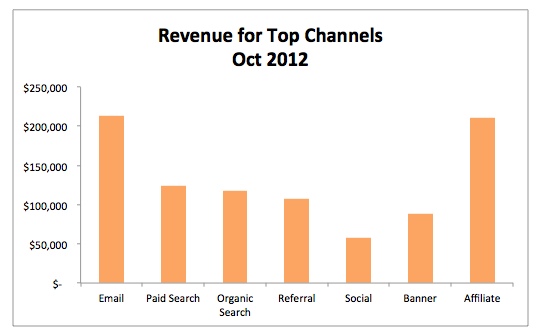
Want to see the difference? Here is an example of the same data sets shown as a pie chart and a bar chart:

Bar charts (resembling a histogram rotated horizontally) are good at showing trend changes over time. You can track multiple values ​​in a given period of time, but the key to understanding a bar chart is the time component.

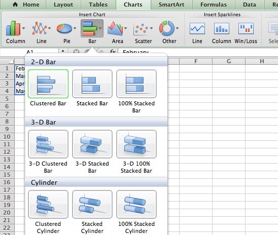
To turn an existing data set into one of these charts in Excel, select the desired data, then open the menu section Diagrams (Charts). В Windows: Insert (Insert) > Diagrams (Charts). Next, select the chart type that best suits your dataset

2. Sort data for a histogram to make it clearer

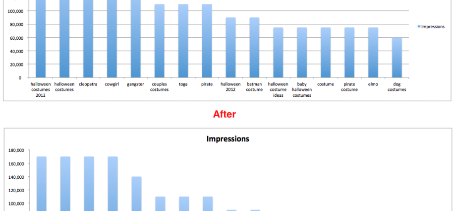
If a histogram is chosen for data visualization, then this technique can significantly affect the result. Most often we see the following histograms:

They are chaotic! You need to spend precious time to understand what data falls out of the big picture. Instead, it was just a matter of ordering the values ​​from largest to smallest. Here’s what it should look like:

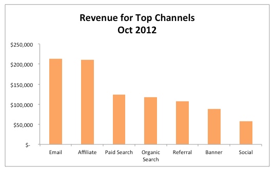
In the case of a bar chart, place the larger values ​​on top. If this is a histogram, then let the values ​​decrease from left to right. Why? Because in this direction we read in (as well as in most European ones). If the chart is intended for a backwards reading audience, change the order in which the data is presented on the chart.

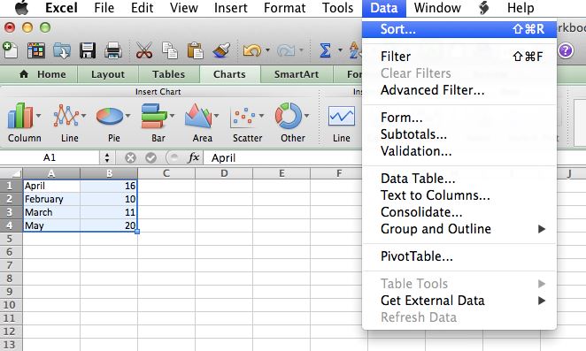
To change the order in which data is presented on a graph, you need to sort them from largest to smallest. On the menu Data (Data) click Sorting (Sort) and select the mode you want.

3. Shorten Y-Axis Labels

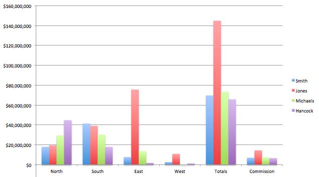
Long Y-axis labels, like large numbers, take up a lot of space and can be confusing at times. For example, as in the diagram below:

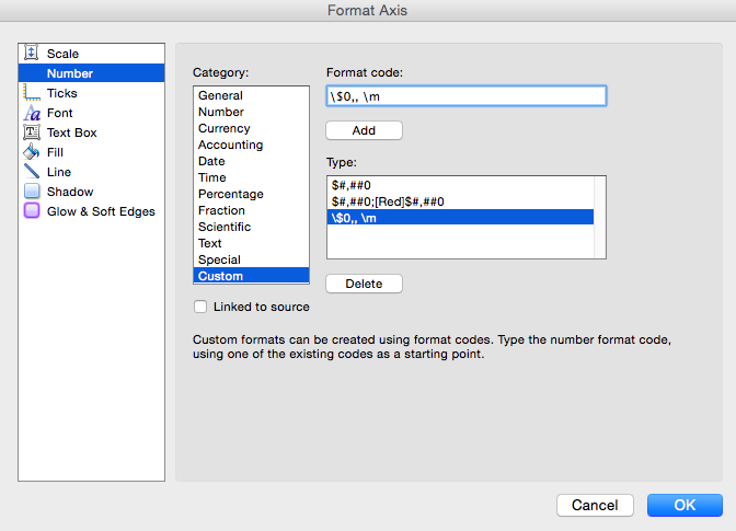
To make them smaller, right-click on one of the labels on the Y-axis and select from the menu that appears. Axis Format (Format Axis). In the menu that opens, go to the section Number (Number) and in the list Category (Category) select Additional (Custom). Uncheck Link to source (Linked to Source) if available, otherwise option Additional (Custom) will be unavailable.

Enter format code $0,, m (as shown in the picture below) and click OK.

As a result, the chart will look much neater:

4. Remove background lines

The graph allows you to make a rough comparison of the data without going into details. No one goes to a chart to see the exact difference between the points – everyone wants the big picture, the main trends.

To help people focus on these trends, remove the background lines from the chart. These lines are completely useless and confusing. Remove them, let people focus on what really matters.

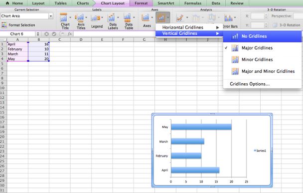
To remove background lines, click chart layout (Chart Layout) > Grid lines (Gridlines) and select No grid lines (No Gridlines) for vertical and horizontal lines.

5. Remove standard indents before the chart

If you don’t manually remove them, Excel will automatically add padding before the first data point and after the last data point, as you can see in the figure below on the left. In the figure on the right, the graph looks much better without these paddings:

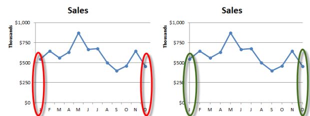
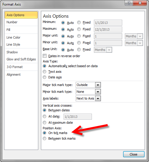
To remove padding, select the horizontal axis, open the menu Axis Format (Format Axis), under Axis parameters (Axis Options) change the parameter Axis position (Position Axis) на Matches divisions. (On Tick Marks).

6. Remove unnecessary formatting

Standard Excel charts usually come with customized styles – but these styles often make it difficult to perceive information. Shadows? contours? Turns? Get rid of it all! They do not add information to the diagram.

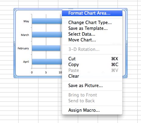
To correct the appearance settings in Excel, right-click on the graph and select Construction area format (Format Chart Area). Remove all unnecessary effects.

7. Avoid 3-D Effects

This advice logically follows from the previous one, but I want to separate it into a separate point, since 3-D effects are overused too often.

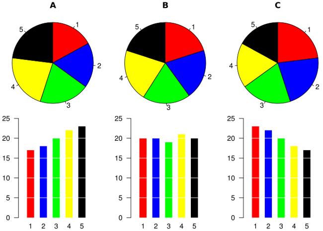
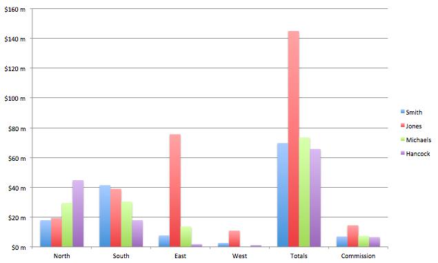
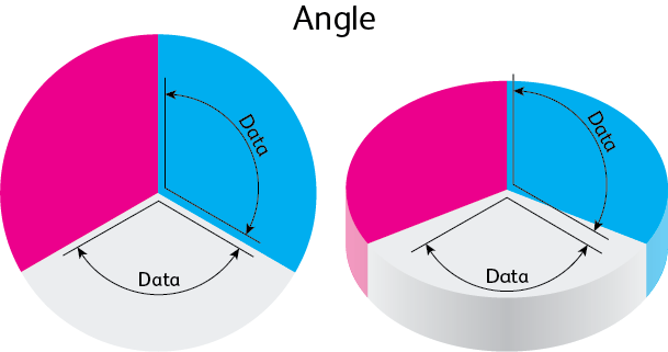
In an effort to make the data look super cool, people often opt for bar, bar, and pie charts with 3-D effects. As a result, it becomes harder to perceive such information. The slope of the graph gives the reader a distorted view of the data. Since the main purpose of diagrams is to tell the reader a detailed story, we don’t want to weaken arguments with bad design. See how the same pie chart looks different in 2-D and 3-D:

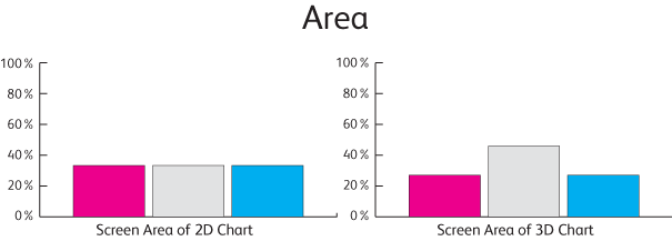
If you evaluate the area that each section actually occupies on the screen, it becomes clear why it is so easy to misunderstand a 3-D diagram:

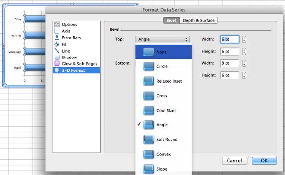
To remove 3-D effects from a graph element, select the element, then under XNUMXD Shape Format (3D Format) set to parameters Relief from above (Top) and Relief from below (Bottom) meaning Without relief (None).

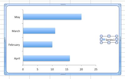
8. Remove the legend if it is not needed

The legend provides information that, as a rule, is easy to understand from the graph even without it. The legend becomes useful when the chart shows a lot of categories on the x-axis, or a lot of data points for each category. But if several points are compared on the chart, then the legend becomes useless. In this case, we delete the legend without hesitation for a long time.

To delete a legend in Excel, you need to select it and click Delete on keyboard.

9. Use personal colors

The colors offered in Excel are rather faded. The easiest way to fix this is to use your signature colors. Thanks to this, the diagram will look much nicer and neater.

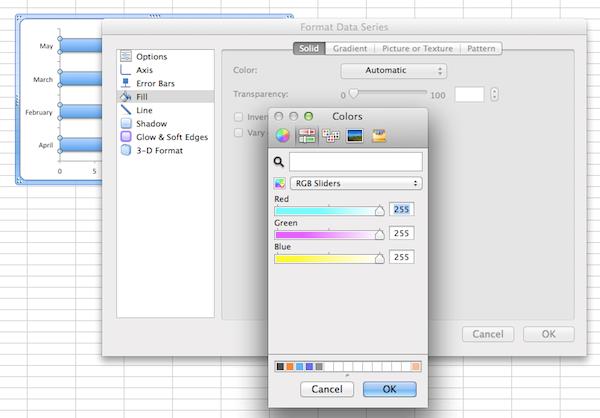
To use the correct colors, you need to use the HEX codes for these colors. Using a converter, convert the color from HEX encoding to RGB. In Excel, double-click on the graph element whose color you want to change. On the menu Data series format (Format data series) under Fill (Fill) select solid fill (Color) > Other colors (More Colors).

In the window that appears, click the second icon from the left with sliders. See the dropdown? Select RGB in it and enter the recently received digital codes. Voila! Great corporate colors and chic graphics!

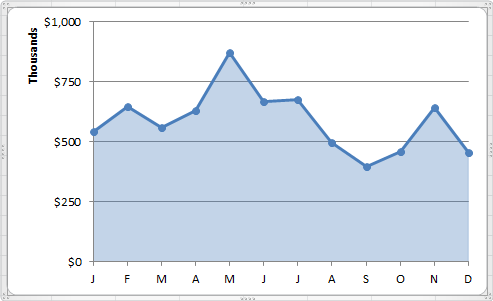
10. Add Shaded Area to Line Chart

Have you ever seen a line chart with a shading area under the line of the graph? This trick will make your line chart stand out from the rest.

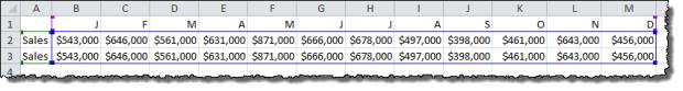
To get this shaded area, you need to trick Excel by adding another data series. To do this, go back to the Excel spreadsheet you used to plot the graph and highlight the data points plotted along the y-axis (in our case, these are dollar amounts). Copy them to the line below so that you get two identical rows of data.

Next, highlight the values ​​of these two identical data series, excluding the labels. In the figure below, this range is outlined in blue.

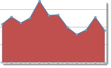
A line of a different color (in our case, red) will appear on top of the original line on the chart. Select this line with a mouse click, then right-click on it and select from the context menu Change the chart type for a series (Change Series Chart Type).

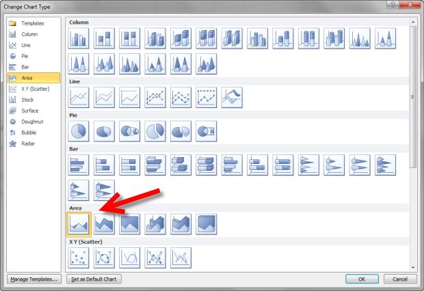
In the menu that opens, select the first chart option from the type with areas (Area).

The new chart will look something like this:

Double-click on the shaded area of ​​the graph (in our case, the red area), a menu will appear Data series format (Format Data Series). In chapter Fill (Fill) select solid fill (solid fill). On the menu Fill color (Fill color) select the same color as the one set for the graph line. Transparency can be set to your liking – a fill that is 66% transparent looks quite good.

Then in the section Border (Border color) select solid line (solid fill). On the menu Outline color (Fill color) select the same color as the one set for the graph line. Set the transparency level of the border to the same as for the fill. Voila, look at the result!

That’s all. Thank you for your attention!