


Contents
Pivot tables is one of the most powerful tools in Excel. They allow you to analyze and sum up various summaries of large amounts of data with just a few mouse clicks. In this article, we will get acquainted with pivot tables, understand what they are, learn how to create and customize them.
This article was written using Excel 2010. The concept of PivotTables has not changed much over the years, but the way you create them is slightly different in each new version of Excel. If you have a version of Excel not 2010, then be prepared that the screenshots in this article will differ from what you see on your screen.
A bit of history
In the early days of spreadsheet software, the Lotus 1-2-3 rule ball. Its dominance was so complete that Microsoft’s efforts to develop its own software (Excel) as an alternative to Lotus seemed like a waste of time. Now fast forward to 2010! Excel dominates spreadsheets more than Lotus code has ever done in its history, and the number of people who still use Lotus is close to zero. How could this happen? What was the reason for such a dramatic turn of events?
Analysts identify two main factors:
- First, Lotus decided that this newfangled GUI platform called Windows was just a passing fad that wouldn’t last long. They refused to build a Windows version of Lotus 1-2-3 (but only for a few years), predicting that the DOS version of their software would be all consumers would ever need. Microsoft naturally developed Excel specifically for Windows.
- Second, Microsoft introduced a tool in Excel called PivotTables that was not available in Lotus 1-2-3. PivotTables, exclusive to Excel, proved to be so overwhelmingly useful that people tended to stick with the new Excel software suite rather than continue with Lotus 1-2-3, which didn’t have them.
PivotTables, along with underestimating the success of Windows in general, played the death march for Lotus 1-2-3 and ushered in the success of Microsoft Excel.
What are pivot tables?
So, what is the best way to characterize what PivotTables are?
In simple terms, pivot tables are summaries of some data, created to facilitate the analysis of this data. Unlike manually created totals, Excel PivotTables are interactive. Once created, you can easily modify them if they don’t give the picture you were hoping for. With just a couple of mouse clicks, totals can be flipped so that column headings become row headings and vice versa. You can do many things with pivot tables. Instead of trying to describe in words all the features of pivot tables, it’s easier to demonstrate it in practice …
The data you analyze with PivotTables cannot be random. It should be raw raw data, like a list of some kind. For example, it could be a list of sales made by the company in the last six months.
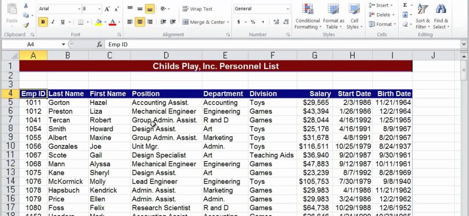
Look at the data shown in the figure below:
Note that this is not raw raw data, as it has already been summarized. In cell B3 we see $30000, which is probably the total result that James Cook did in January. Where is the original data then? Where did the $30000 figure come from? Where is the original list of sales from which this monthly total was derived? It is clear that someone has done a great job of organizing and sorting all the sales data for the last six months and turning it into the table of totals that we see. How long do you think it took? Hour? Ten o’clock?
The fact is that the table above is not a pivot table. It was hand-crafted from raw data stored elsewhere and took at least a couple of hours to process. Just such a summary table can be created using pivot tables in just a few seconds. Let’s figure out how…
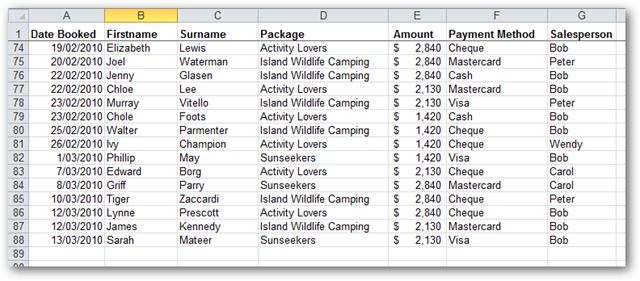
If we go back to the original sales list, it would look something like this:

You might be surprised that from this list of trades with the help of pivot tables and in just a few seconds, we can create a monthly sales report in Excel, which we analyzed above. Yes, we can do that and more!
How to create a pivot table?
First, make sure you have some source data in an Excel sheet. The list of financial transactions is the most typical that occurs. In fact, it could be a list of anything: employee contact details, a CD collection, or your company’s fuel consumption data.
So, we start Excel … and load such a list …
After we have opened this list in Excel, we can start creating a pivot table.
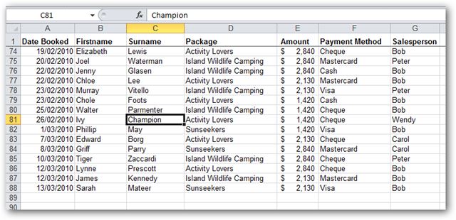
Select any cell from this list:
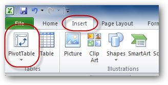
Then on the tab Insertion (Insert) select command PivotTable (Pivot table):
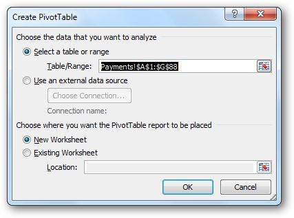
A dialog box will appear Create PivotTable (Creating a pivot table) with two questions for you:
- What data to use to create a new pivot table?
- Where to put the pivot table?
Since in the previous step we have already selected one of the list cells, the entire list will be automatically selected to create a pivot table. Note that we can select a different range, a different table, and even some external data source such as an Access or MS-SQL database table. In addition, we need to choose where to place the new pivot table: on a new sheet or on one of the existing ones. In this example, we will choose the option – New Worksheet (to a new sheet):
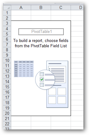
Excel will create a new sheet and place an empty pivot table on it:
As soon as we click on any cell in the pivot table, another dialog box will appear: PivotTable Field List (Pivot table fields).
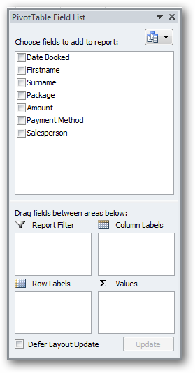
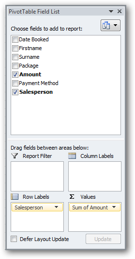
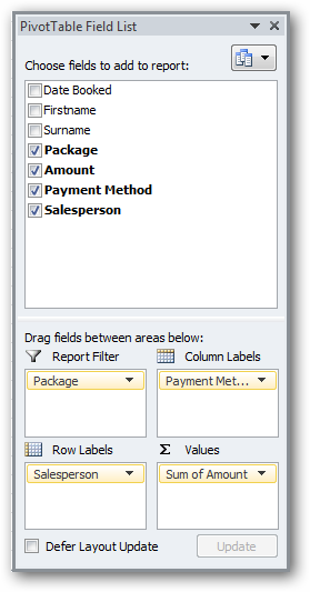
The list of fields at the top of the dialog box is a list of all the titles from the original list. The four empty areas at the bottom of the screen allow you to tell the PivotTable how you want to summarize the data. As long as these areas are empty, there is nothing in the table either. All we have to do is drag the headings from the top area to the empty areas below. At the same time, a pivot table is automatically generated, in accordance with our instructions. If we make a mistake, we can remove the headings from the bottom area or drag others to replace them.
Area Values (Meanings) is probably the most important of the four. Which heading is placed in this area determines what data will be summarized (sum, average, maximum, minimum, etc.) These are almost always numerical values. An excellent candidate for a place in this area is the data under the heading Amount (Cost) of our original table. Drag this title to the area Values (Values):
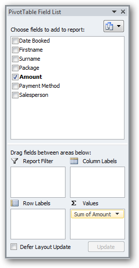
Please note that the title Amount is now marked with a checkmark, and in the area Values (Values) an entry has appeared Sum of Amount (Amount field Amount), indicating that the column Amount summed up.
If we look at the pivot table itself, we will see the sum of all values from the column Amount original table.
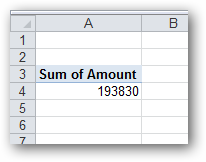
So, our first pivot table is created! Convenient, but not particularly impressive. We probably want to get more information about our data than we currently have.
Let’s turn to the original data and try to identify one or more columns that can be used to split this sum. For example, we can form our pivot table in such a way that the total amount of sales is calculated for each seller individually. Those. rows will be added to our pivot table with the name of each salesperson in the company and their total sales amount. To achieve this result, just drag the title sales person (sales representative) to the region Row Labels (Strings):
It becomes more interesting! Our PivotTable is starting to take shape…
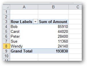
See the benefits? In a couple of clicks, we created a table that would have taken a very long time to create manually.
What else can we do? Well, in a sense, our pivot table is ready. We have created a useful summary of the original data. Important information already received! In the rest of this article, we’ll look at some ways to create more complex PivotTables, as well as learn how to customize them.
PivotTable Setup
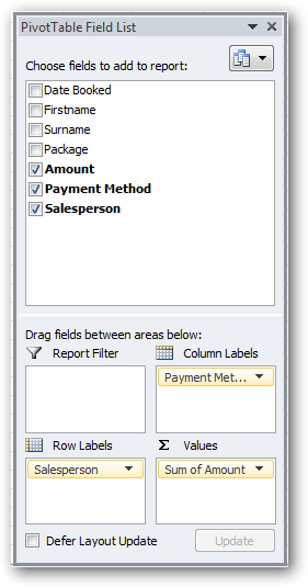
First, we can create a two-dimensional pivot table. Let’s do this using the column heading Payment Method (Payment method). Just drag the title Payment Method to the area Column Labels (Columns):
We get the result:
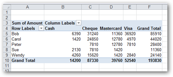
Looks very cool!
Now let’s make a three-dimensional table. What would such a table look like? Let’s see…
Drag Header Package (Complex) to the area report filters (Filters):
Note where he is…
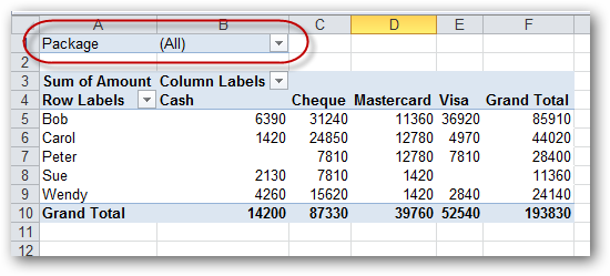
This gives us the opportunity to filter the report on the basis of “Which holiday complex was paid for.” For example, we can see a breakdown by sellers and by payment methods for all complexes, or in a couple of mouse clicks, change the view of the pivot table and show the same breakdown only for those who ordered the complex Sunseekers.
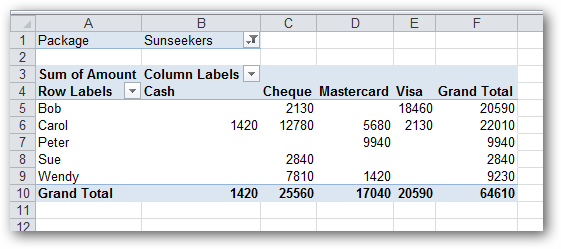
So, if you understand this correctly, then our pivot table can be called three-dimensional. Let’s continue setting up…
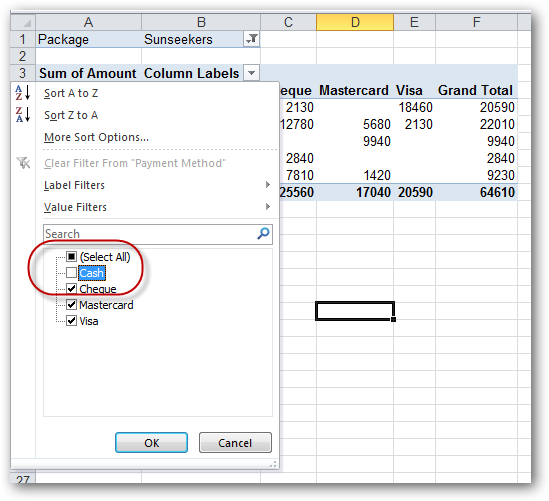
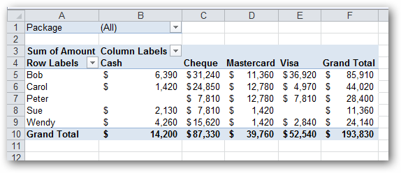
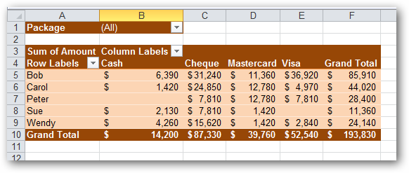
If it suddenly turns out that only payment by check and credit card (that is, cashless payment) should be displayed in the pivot table, then we can turn off the display of the title Cash (Cash). For this, next to Column Labels click the down arrow and uncheck the box in the drop-down menu Cash:
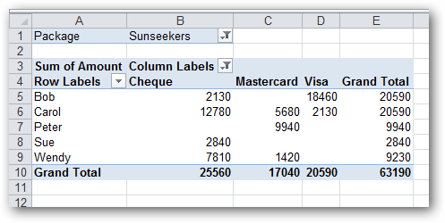
Let’s see what our pivot table looks like now. As you can see, the column Cash disappeared from her.
Formatting PivotTables in Excel
PivotTables are obviously a very powerful tool, but so far the results look a little plain and boring. For example, the numbers we add up don’t look like dollar amounts – they’re just numbers. Let’s fix this.
It is tempting to do what you are used to in such a situation and simply select the entire table (or the entire sheet) and use the standard number formatting buttons on the toolbar to set the desired format. The problem with this approach is that if you ever change the structure of the pivot table in the future (which happens with a 99% chance), the formatting will be lost. What we need is a way to make it (almost) permanent.
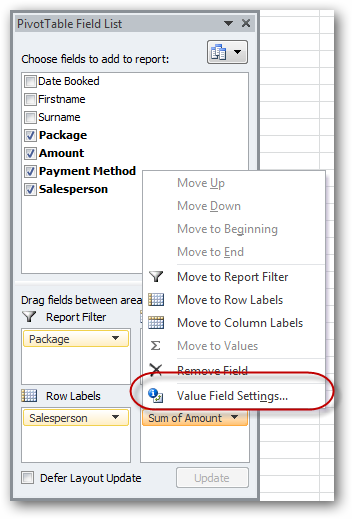
First, let’s find the entry Sum of Amount in Values (Values) and click on it. In the menu that appears, select the item Value Field Settings (Value field options):
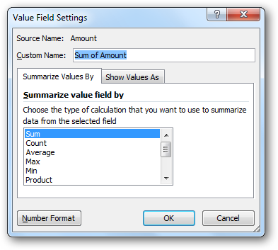
A dialog box will appear Value Field Settings (Value field options).
Нажмите кнопку Number Format (Number Format), a dialog box will open. Format Cells (cell format):
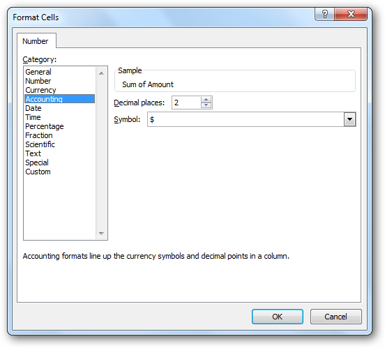
From the list Category (Number formats) select Accounting (Financial) and set the number of decimal places to zero. Now press a few times OKto go back to our pivot table.
As you can see, the numbers are formatted as dollar amounts.
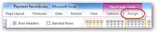
While we’re at it with formatting, let’s set up the format for the entire PivotTable. There are several ways to do this. We use the one that is simpler …
Click the PivotTable Tools: Design (Working with PivotTables: Constructor):
Next, expand the menu by clicking on the arrow in the lower right corner of the section PivotTable Styles (PivotTable Styles) to see the extensive collection of inline styles:
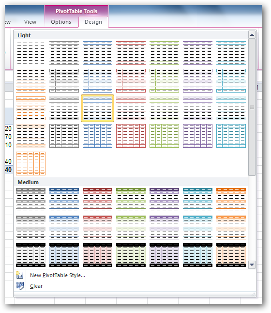
Choose any suitable style and look at the result in your pivot table:
Other PivotTable Settings in Excel
Sometimes you need to filter data by dates. For example, in our list of trades there are many, many dates. Excel provides a tool to group data by day, month, year, and so on. Let’s see how it’s done.
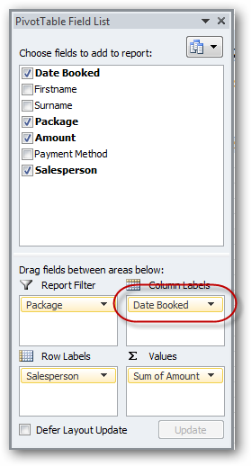
First remove the entry. Payment Method from the region Column Labels (Columns). To do this, drag it back to the list of titles, and in its place, move the title Date Booked (date of booking):
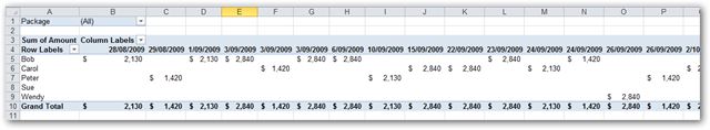
As you can see, this temporarily rendered our pivot table useless. Excel created a separate column for each date on which a trade was made. As a result, we got a very wide table!
To fix this, right-click on any date and select from the context menu GROUP (Group):
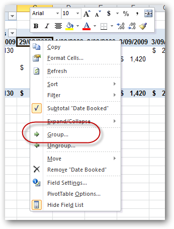
The grouping dialog box will appear. We choose Months (Months) and click OK:
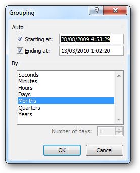
Voila! This table is much more useful:
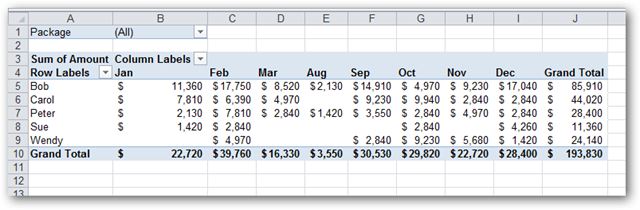
By the way, this table is almost identical to the one shown at the beginning of the article, where the sales totals were compiled manually.
There is another very important point that you need to know! You can create not one, but several levels of row (or column) headings:
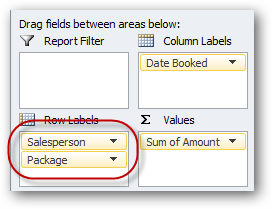
… and it will look like this …
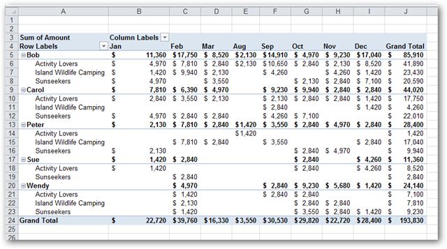
The same can be done with column headings (or even filters).
Let’s return to the original form of the table and see how to display averages instead of sums.
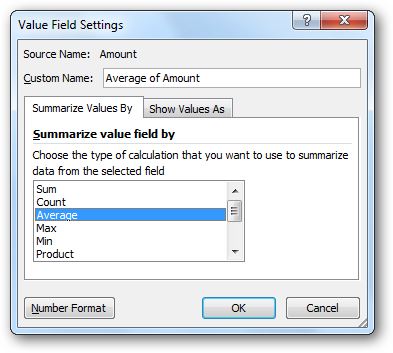
To get started, click on Sum of Amount and from the menu that appears select Value Field Settings (Value field options):

The list Summarize value field by (Operation) in the dialog box Value Field Settings (Value field options) select Average (Average):
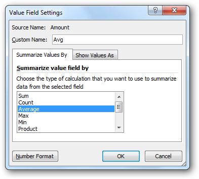
At the same time, while we are here, let’s change CustomName (Custom name) with Average of Amount (Amount field Amount) to something shorter. Enter in this field something like Avg:
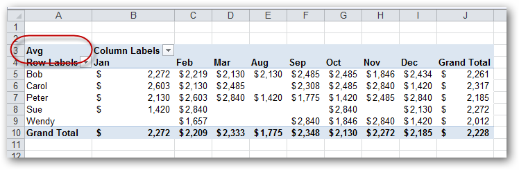
Press OK and see what happens. Note that all values have changed from totals to averages, and the table header (in the upper left cell) has changed to Avg:
If you want, you can immediately get the amount, average and number (sales) placed in one pivot table.
Here is a step by step guide on how to do this, starting with an empty pivot table:
- Drag Header sales person (sales representative) to the region Column Labels (Columns).
- Drag the title three times Amount (Cost) to area Values (Values).
- For the first field Amount change the title to Total (Amount), and the number format in this field is Accounting (Financial). The number of decimal places is zero.
- Second field Amount name Average, set the operation for it Average (Average) and the number format in this field also change to Accounting (Financial) with zero decimal places.
- For the third field Amount set a title Count and an operation for him – Count (Quantity)
- In the Column Labels (Columns) field automatically created Σ Values (Σ Values) – drag it to the area Row Labels (Lines)
Here is what we will end up with:
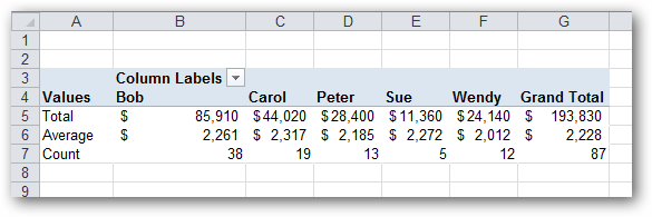
Total amount, average value and number of sales – all in one pivot table!
Conclusion
Pivot tables in Microsoft Excel contain a lot of features and settings. In such a small article, they are not even close to cover them all. It would take a small book or a large website to fully describe all the possibilities of pivot tables. Bold and inquisitive readers can continue their exploration of pivot tables. To do this, just right-click on almost any element of the pivot table and see what functions and settings open. On the Ribbon you will find two tabs: PivotTable Tools: Options (analysis) and Design (Constructor). Don’t be afraid to make a mistake, you can always delete the PivotTable and start over. You have an opportunity that long time users of DOS and Lotus 1-2-3 never had.