Contents
In this tutorial you will find some interesting examples demonstrating how to use the function VPR (VLOOKUP) along with SUM (SUM) or SUMMESLI (SUMIF) in Excel to search and sum values based on one or more criteria.
Are you trying to create a summary file in Excel that will identify all instances of one particular value and sum the other values associated with it? Or do you need to find all values in an array that meet a given condition and then sum the related values from another sheet? Or perhaps you have an even more difficult task, such as looking through a table of all your company’s invoices, finding among them the invoices of a certain seller and summing them up?
The tasks may differ, but their meaning is the same – you need to find and sum the values uXNUMXbuXNUMXbof one or more criteria in Excel. What are these values? Any number. What are these criteria? Any… From a number or a cell reference containing the desired value to logical operators and Excel formula results.
So, is there any functionality in Microsoft Excel that can cope with the tasks described? Of course! The solution lies in the combination of functions VPR (VLOOKUP) or VIEW (LOOKUP) with functions SUM (SUM) or SUMMESLI (SUMIF). The formula examples below will help you understand how these functions work and how to use them with real data.
Please note that the examples provided are designed for an advanced user who is familiar with the basic principles and syntax of the function. VPR. If you are still far from this level, we recommend that you pay attention to the first part of the tutorial – VLOOKUP function in Excel: syntax and examples.
VLOOKUP and SUM in Excel – calculate the sum of the found matching values
If you work with numeric data in Excel, then quite often you have to not only extract related data from another table, but also sum several columns or rows. To do this, you can combine the functions SUM и VPR, as shown below.
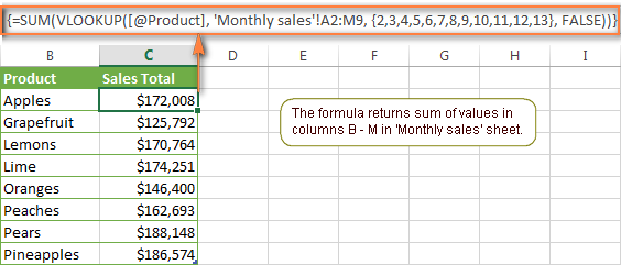
Let’s say we have a list of products with several months of sales data, with a separate column for each month. Data Source – Sheet Monthly Sales:
Now we need to make a table of totals with the amounts of sales for each product.
The solution to this problem is to use an array of constants in the argument col_index_num (column_number) functions VPR. Here is an example formula:
=SUM(VLOOKUP(lookup value, lookup range, {2,3,4}, FALSE))
=СУМ(ВПР(искомое_значение;таблица;{2;3;4};ЛОЖЬ))
As you can see we have used an array 2,3,4 {} for the third argument to search multiple times in the same function VPR, and get the sum of the values in the columns 2, 3 и 4.
Now let’s apply this combination VPR и SUM to the data in our table to find the total amount of sales in columns with B by M:
=SUM(VLOOKUP(B2,'Monthly sales'!$A$2:$M$9,{2,3,4,5,6,7,8,9,10,11,12,13},FALSE))
=СУМ(ВПР(B2;'Monthly sales'! $A$2:$M$9;{2;3;4;5;6;7;8;9;10;11;12;13};ЛОЖЬ))
Important! If you are entering an array formula, be sure to press the combination Ctrl + Shift + Enter instead of normal pressing Enter. Microsoft Excel will enclose your formula in curly braces:
{=SUM(VLOOKUP(B2,'Monthly sales'!$A$2:$M$9,{2,3,4,5,6,7,8,9,10,11,12,13},FALSE))}
{=СУМ(ВПР(B2;'Monthly sales'!$A$2:$M$9;{2;3;4;5;6;7;8;9;10;11;12;13};ЛОЖЬ))}
If we limit ourselves to a simple click Enter, the calculation will be performed only on the first value of the array, which will lead to an incorrect result.
You might be wondering why the formula in the figure above displays [@Product]as the desired value. This is because my data was converted to a table using the command Table (Table) tab Insertion (Insert). I’m more comfortable working with full-featured Excel spreadsheets than simple ranges. For example, when you enter a formula in one of the cells, Excel automatically copies it to the entire column, saving you a few precious seconds.
As you can see, use the functions VPR и SUM in Excel is quite simple. However, this is far from an ideal solution, especially if you have to work with large tables. The fact is that using array formulas can slow down the application, since each value in the array makes a separate function call. VPR. It turns out that the more values in the array, the more array formulas in the workbook and the slower Excel works.
This problem can be overcome by using a combination of functions INDEX (INDEX) and MATCH (POISKPOZ) instead VLOOKUP (VLOOKUP) and SUM (SUM). Later in this article you will see some examples of such formulas.
Performing other calculations using the VLOOKUP function in Excel
We just looked at an example of how you can extract values from several columns of a table and calculate their sum. In the same way, you can perform other mathematical operations on the results returned by the function. VPR. Here are some examples of formulas:
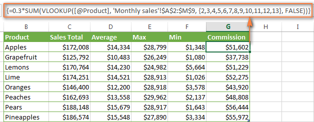
We calculate the average:
{=AVERAGE(VLOOKUP(A2,'Lookup Table'!$A$2:$D$10,{2,3,4},FALSE))}
{=СРЗНАЧ(ВПР(A2;'Lookup Table'!$A$2:$D$10;{2;3;4};ЛОЖЬ))}
The formula looks up the value from cell A2 in the worksheet Lookup table and calculates the arithmetic mean of the values that are at the intersection of the found row and columns B, C, and D.
Finding the maximum:
{=MAX(VLOOKUP(A2,'Lookup Table'!$A$2:$D$10,{2,3,4},FALSE))}
{=МАКС(ВПР(A2;'Lookup Table'!$A$2:$D$10;{2;3;4};ЛОЖЬ))}
The formula looks up the value from cell A2 in the worksheet Lookup table and returns the maximum of the values that are at the intersection of the found row and columns B, C, and D.
Finding the minimum:
{=MIN(VLOOKUP(A2,'Lookup Table'!$A$2:$D$10,{2,3,4},FALSE))}
{=МИН(ВПР(A2;'Lookup Table'!$A$2:$D$10;{2;3;4};ЛОЖЬ))}
The formula looks up the value from cell A2 in the worksheet Lookup table and returns the minimum of the values that are at the intersection of the found row and columns B, C, and D.
We calculate % of the amount:
{=0.3*SUM(VLOOKUP(A2,'Lookup Table'!$A$2:$D$10,{2,3,4},FALSE))}
{=0.3*СУММ(ВПР(A2;'Lookup Table'!$A$2:$D$10;{2;3;4};ЛОЖЬ))}
The formula looks up the value from cell A2 in the worksheet Lookup table, then sums the values that are at the intersection of the found row and columns B, C and D, and only then calculates 30% of the sum.
If we add the formulas listed above to the table from the previous example, the result will look like this:
In the case where your desired value is an array, the function VPR becomes useless because it does not know how to work with data arrays. In such a situation, you can use the function VIEW (LOOKUP) in Excel, which is similar to VPR, and it works with arrays in the same way as with single values.
Let’s look at an example to make it clearer what we are talking about. Suppose we have a table that lists the names of customers, purchased items and their quantities (table Main table). In addition, there is a second table containing the prices of goods (Lookup table). Our task is to write a formula that will find the sum of all orders of a given customer.
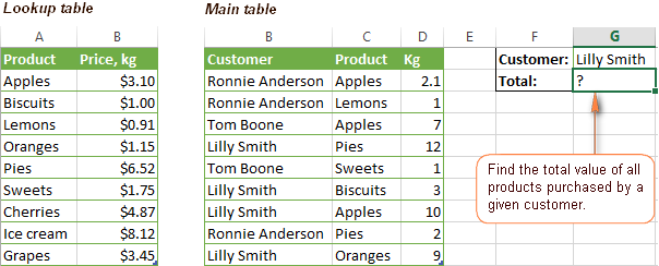
As you remember, you cannot use the function VPRif the lookup value occurs multiple times (it’s an array of data). Use a combination of functions instead SUM и VIEW:
=SUM(LOOKUP($C$2:$C$10,'Lookup table'!$A$2:$A$16,'Lookup table'!$B$2:$B$16)*$D$2:$D$10*($B$2:$B$10=$G$1))
=СУММ(ПРОСМОТР($C$2:$C$10;'Lookup table'!$A$2:$A$16;'Lookup table'!$B$2:$B$16)*$D$2:$D$10*($B$2:$B$10=$G$1))
Since this is an array formula, don’t forget to press the combination Ctrl + Shift + Enter when input is completed.
Lookup table is the name of the sheet where the view range is located.
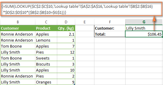
Let’s break down the ingredients of the formula so you understand how it works and can customize it to suit your needs. Function SUM let’s leave it aside for now, since its purpose is obvious.
LOOKUP($C$2:$C$10,'Lookup table'!$A$2:$A$16,'Lookup table'!$B$2:$B$16)ПРОСМОТР($C$2:$C$10;'Lookup table'!$A$2:$A$16;'Lookup table'!$B$2:$B$16)Function VIEW looks up the products listed in column C of the Main table and returns the corresponding price from column B of the lookup table.
- $D$2:$D$10 – the number of goods purchased by each customer whose name is in column D of the main table. Multiplying the quantity of an item by the price returned by the function VIEW, we get the cost of each purchased product.
- $B$2:$B$10=$G$1 – The formula compares the customer names in column B of the main table with the name in cell G1. If there is a match, return 1, otherwise 0. Thus, customer names that differ from those specified in cell G1 are discarded, because we all know that multiplication by zero gives zero.
Since our formula is an array formula, it repeats the steps above for each value in the lookup array. Finally, the function SUM calculates the sum of the values resulting from the multiplication. Not difficult at all, do you agree?
Comment. To function VIEW worked correctly, the viewed column should be sorted in ascending order.
VLOOKUP and SUMIF – find and sum values that satisfy a certain criterion
Function SUMMESLI (SUMIF) in Excel is similar to SUM (SUM), which we just discussed, because it also sums the values. The only difference is that SUMMESLI sums only those values that meet the criteria you specify. For example, the simplest formula with SUMMESLI:
=SUMIF(A2:A10,">10")
=СУММЕСЛИ(A2:A10;">10")
– sums all cell values in a range A2: A10, which are more 10.
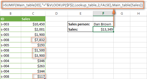
Very simple, right? Now let’s look at a slightly more complex example. Suppose we have a table that lists the names of sellers and their numbers ID (lookup table). In addition, there is another table in which the same ID linked to sales data (Main table). Our task is to find the amount of sales for a given seller. There are 2 aggravating circumstances here:
- Main table contains many records for one ID in random order.
- You cannot add a vendor name column to the main table.
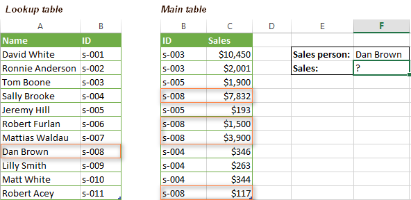
Let’s write a formula that will find all the sales made by a given salesperson and also sum up the found values.
Before we start, let me remind you the syntax of the function SUMMESLI (SUMIF):
SUMIF(range,criteria,[sum_range])
СУММЕСЛИ(диапазон;критерий;[диапазон_суммирования])
- range (range) – the argument speaks for itself. It’s just a range of cells that you want to evaluate by the given criteria.
- Criteria (criteria) is a condition that tells the formula which values to sum. Can be a number, cell reference, expression, or another Excel function.
- sum_range (summation_range) is an optional but very important argument for us. It defines the range of related cells that will be summed. If it is not specified, Excel sums the cell values in the first argument to the function.
Putting it all together, let’s define the third argument for our function SUMMESLI. As you remember, we want to sum up all the sales made by a particular seller whose name is given in cell F2 (see the figure above).
- range (range) – since we are looking for ID seller, the values of this argument will be the values in column B of the Main table. You can set the range B:B (whole column) or, converting the data to a table, use the column name Main_table[ID].
- Criteria (criteria) – since the names of sellers are recorded in the lookup table (Lookup table), we use the function VPR For search ID, corresponding to the given seller. The name is written in cell F2, so for the search we use the formula:
VLOOKUP($F$2,Lookup_table,2,FALSE)ВПР($F$2;Lookup_table;2;ЛОЖЬ)Of course, you could enter the name as a lookup value directly into the function VPR, but it’s better to use an absolute cell reference, because this way we create a universal formula that will work for any value entered in this cell.
- sum_range (summation_range) is the easiest part. Since the sales data is recorded in column C, which is called Sales, then we just write Main_table[Sales].
All you have to do is combine the parts into one whole, and the formula SUMIF+VLOOKUP will be ready:
=SUMIF(Main_table[ID],VLOOKUP($F$2,Lookup_table,2,FALSE),Main_table[Sales])
=СУММЕСЛИ(Main_table[ID];ВПР($F$2;Lookup_table;2;ЛОЖЬ);Main_table[Sales])