One of the most significant advantages of charts in Excel is the ability to compare data series with their help. But before creating a chart, it’s worth spending a little time thinking about what data and how to show it in order to make the picture as clear as possible.
Let’s take a look at ways Excel can display multiple data series to create a clear and easy-to-read chart without resorting to PivotCharts. The described method works in Excel 2007-2013. Images are from Excel 2013 for Windows 7.
Column and bar charts with multiple data series
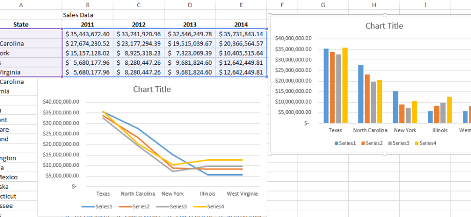
To create a good chart, first check that the data columns have headings and that the data is arranged in the best way to understand it. Make sure all data is scaled and sized the same, otherwise it can get confusing, for example, if one column has sales data in dollars and the other column has millions of dollars.
Select the data you want to show in the chart. In this example, we want to compare the top 5 states by sales. On the tab Insert (Insert) select which chart type to insert. It will look something like this:
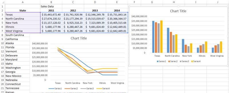
As you can see, it will take a little tidying up the diagram before presenting it to the audience:
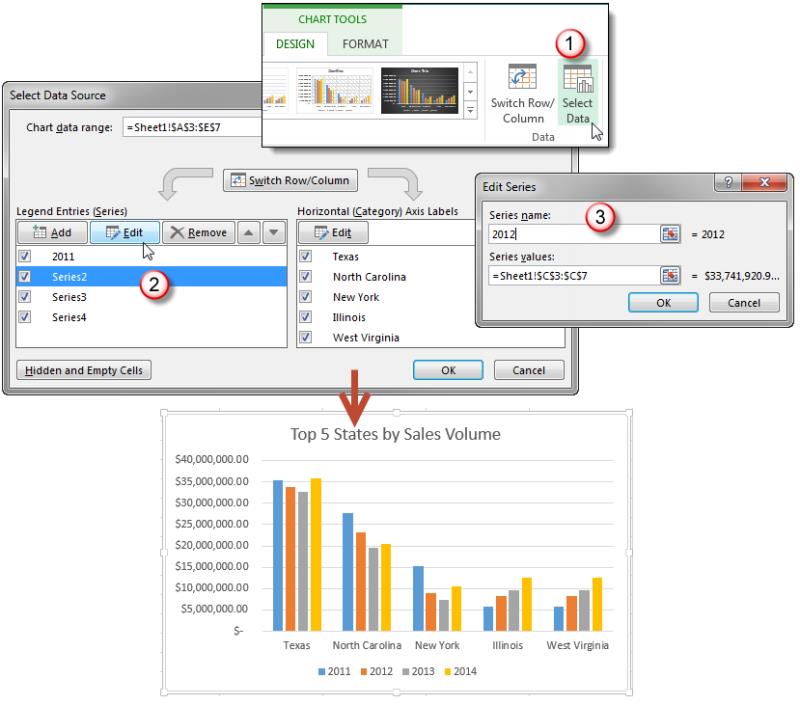
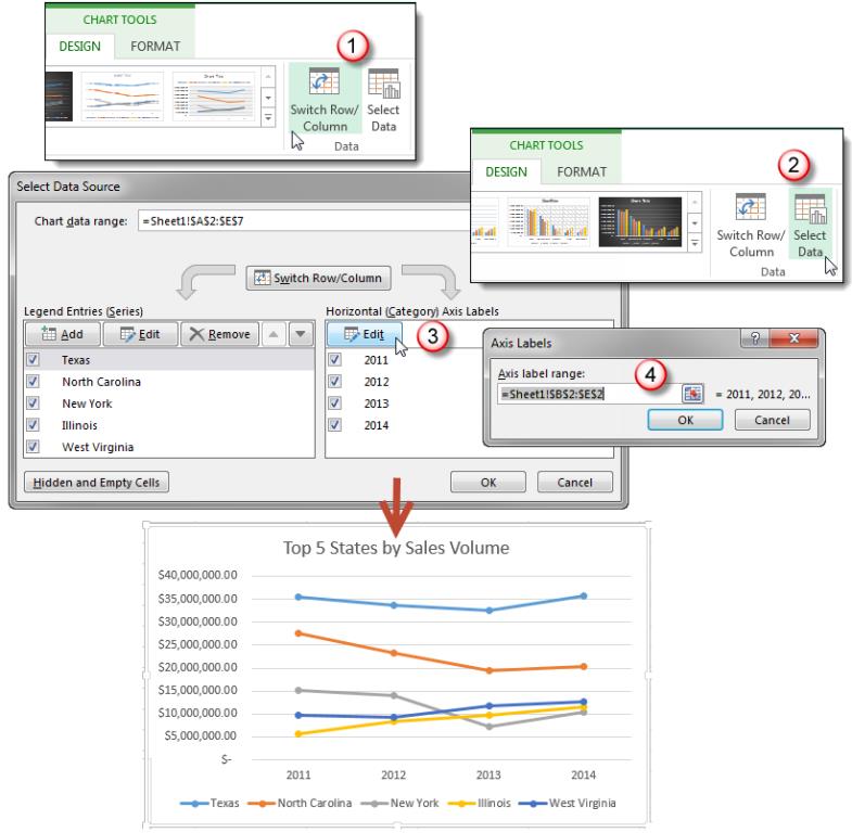
- Add titles and data series labels. Click on the chart to open the tab group Working with charts (Chart Tools), then edit the chart title by clicking on the text field Chart title (Chart Title). To change data series labels, follow these steps:
- Нажмите кнопку Select data (Select Data) tab Constructor (Design) to open the dialog Selecting a data source (Select Data Source).
- Select the data series you want to change and click the button Change (Edit) to open the dialog Row change (Edit Series).
- Type a new data series label in the text field Row name (Series name) and press OK.

- Swap rows and columns. Sometimes a different chart style requires a different arrangement of information. Our standard bar chart makes it hard to see how each state’s results have changed over time. Click the button Row column (Switch Row/Column) on tab Constructor (Design) and add the correct labels for the data series.
Create a combo chart
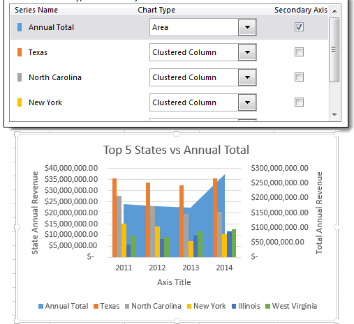
Sometimes you need to compare two dissimilar datasets, and this is best done using different types of charts. The Excel combo chart allows you to display different data series and styles in a single chart. For example, let’s say we want to compare the Annual Total against the sales of the top 5 states to see which states are following the overall trends.
To create a combo chart, select the data you want to show on it, then click the dialog box launcher Inserting a chart (Chart Insert) in the corner of the command group Diagrams (Charts) tab Insert (Insert). In chapter All diagrams (All Charts) click Combined (Combo).
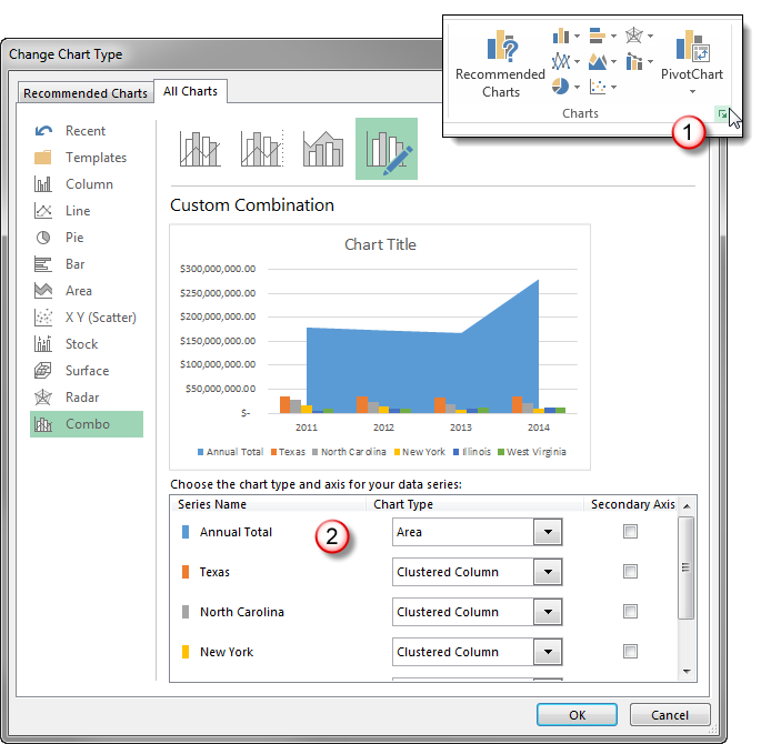
Select the appropriate chart type for each data series from the drop-down lists. In our example, for a series of data Annual Total we chose a chart with areas (Area) and combined it with a histogram to show how much each state contributes to the total and how their trends match.
In addition, the section Combined (Combo) can be opened by pressing the button Change chart type (Change Chart Type) tab Constructor (Design).
Tip: If one of the data series has a different scale from the rest and the data becomes difficult to distinguish, then check the box Secondary axle (Secondary Axis) in front of a row that does not fit into the overall scale.