


Contents
New Chart Wizard
The procedure for constructing charts for a selected range of cells is now significantly simplified thanks to a new dialog box with a preview of the finished chart (both options at once – by rows and by columns):

Combined charts where two or three types are mixed (histogram-plot-with areas, etc.) are now placed in a separate position and are very conveniently configured right away in the Wizard window:

Also now in the chart insertion window there is a tab Recommended charts (Recommended Charts), where Excel will suggest the most suitable chart types based on the type of your initial data:

Suggests, I must say, very competently. In difficult cases, he even suggests using the second axis with its own scale (rubles-percentage), etc. Not bad.
Customizing charts
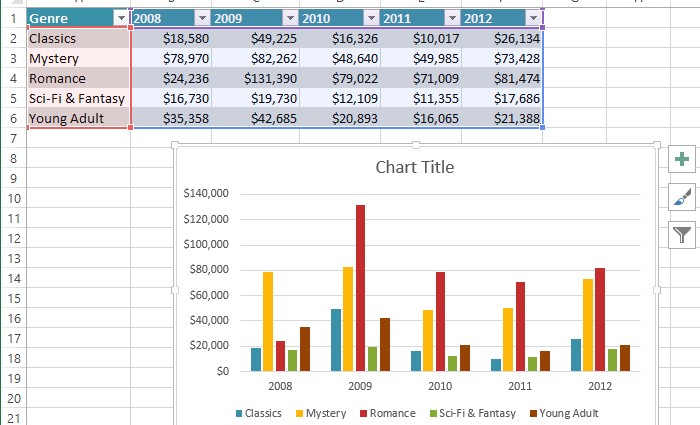
To quickly configure all the basic parameters of any chart, you can now use three key buttons that appear to the right of the selected chart:
- Chart elements (Chart Elements) – allows you to quickly add and customize any chart element (titles, axes, grid, data labels, etc.)
- Chart styles (Chart Styles) – allows the user to quickly select the design and color palette of the diagram from the collection
- Chart Filters (Chart Filters) – allows you to filter the data for the chart on the fly, leaving only the necessary series and categories in it
Everything is conveniently presented in the form of multi-level hierarchical menus, supports on-the-fly preview and works very quickly and conveniently:
If, however, this new customization interface is not to your liking, then you can go the classic way – all the basic operations for customizing the appearance of the chart can also be performed using the tabs Constructor (Design) и Framework (Format). And here are the tabs Layout (Layout), where most chart options were configured in Excel 2007/2010, is no longer there.
Task pane instead of dialog boxes
Fine-tuning the design of each chart element is now very conveniently done using a special panel on the right side of the Excel 2013 window – a task pane that replaces the classic formatting dialog boxes. To display this panel, right-click on any chart element and select the command Framework (Format) or press the keyboard shortcut CTRL + 1 or double-click with the left:

Callout data labels
When adding data labels to selected elements of a chart series, it is now possible to arrange them in callouts automatically snapped to points:

Previously, such callouts had to be drawn manually (that is, simply inserted as separate graphic objects) and, of course, there was no question of any binding to data.
Labels for points from cells
I can’t believe my eyes! Finally, the dream of many users has come true, and the developers have implemented what has been expected of them for almost 10 years – now you can take data labels for the elements of a series of charts directly from the sheet by selecting the option in the task pane Values from cells (Values From Cells) and specifying a range of cells with point labels:

Labels for bubble and scatter charts, any non-standard labels are no longer a problem! What used to be possible only manually (try adding labels to fifty points by hand!) or using special macros / add-ons (XYChartLabeler, etc.), is now a standard Excel 2013 function.
Chart Animation
This new charting feature in Excel 2013, though not a major one, will still add some mojo to your reports. Now, when changing the source data (manually or by recalculating formulas), the diagram will smoothly “flow” into a new state, visually displaying the changes that have occurred:
Trifle, but nice.
- What’s new in Excel 2013 PivotTables