


Contents
From time to time, an Excel user may have the task of turning a range of data that has a horizontal structure into a vertical one. This process is called transposition. This word is new to most people, because in normal PC work you do not have to use this operation. However, those who have to work with large amounts of data need to know how to do it. Today we will talk in more detail about how to perform it, with what function, and also look at some other methods in detail.
TRANSPOSE function – transpose cell ranges in Excel
One of the most interesting and functional table transposition methods in Excel is the function TRANSP. With its help, you can turn a horizontal data range into a vertical one, or perform the reverse operation. Let’s see how to work with it.
Function syntax
The syntax for this function is incredibly simple: TRANSPOSE(array). That is, we need to use only one argument, which is a data set that needs to be converted to a horizontal or vertical view, depending on what it was originally.
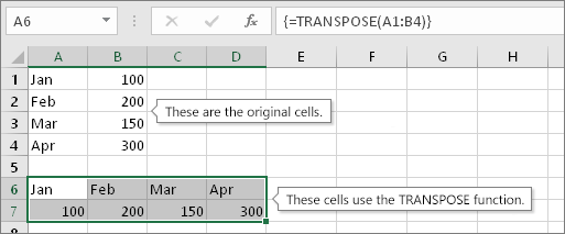
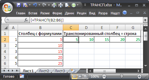
Transposing vertical ranges of cells (columns)
Suppose we have a column with the range B2:B6. They can contain both ready-made values and formulas that return results to these cells. It is not so important for us, transposition is possible in both cases. After applying this function, the row length will be the same as the original range column length.
The sequence of steps for using this formula is as follows:
- Select a line. In our case, it has a length of five cells.
- After that, move the cursor to the formula bar, and enter the formula there =TRANSP(B2:B6).
- Press the key combination Ctrl + Shift + Enter.
Naturally, in your case, you need to specify the range that is typical for your table.
Transposing horizontal cell ranges (rows)
In principle, the mechanism of action is almost the same as the previous paragraph. Suppose we have a string with start and end coordinates B10:F10. It can also contain both directly values and formulas. Let’s make a column out of it, which will have the same dimensions as the original row. The sequence of actions is as follows:
- Select this column with the mouse. You can also use the keys on the keyboard Ctrl and the down arrow, after clicking on the topmost cell of this column.
- After that we write the formula =TRANSP(B10:F10) in the formula bar.
- We write it as an array formula using the key combination Ctrl + Shift + Enter.
Transposing with Paste Special
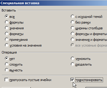
Another possible transposition option is to use the Paste Special function. This is no longer an operator to be used in formulas, but it is also one of the popular methods for turning columns into rows and vice versa.
This option is on the Home tab. To access it, you need to find the “Clipboard” group, and there find the “Paste” button. After that, open the menu that is located under this option and select the “Transpose” item. Before that, you need to select the range that you want to select. As a result, we will get the same range, only the opposite is mirrored.
3 Ways to Transpose a Table in Excel
But in fact, there are much more ways to turn columns into rows and vice versa. Let’s describe 3 methods by which we can transpose a table in Excel. We discussed two of them above, but we will give a few more examples so that you get a better idea of uXNUMXbuXNUMXbhow to carry out this procedure.
Method 1: Paste Special
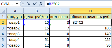
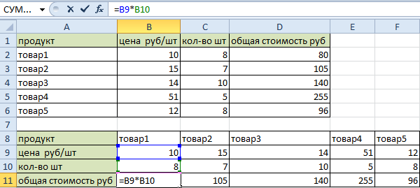
This method is the simplest. It is enough to press a couple of buttons, and the user receives a transposed version of the table. Let’s give a small example for greater clarity. Suppose we have a table containing information about how many products are currently in stock, as well as how much they cost in total. The table itself looks like this.

We see that we have a header and a column with product numbers. In our example, the header contains information about what product, how much it costs, how much it is in stock, and what is the total cost of all products related to this item that are in stock. We get the cost according to the formula where the cost is multiplied by the quantity. To make the example more visual, let’s make the header green.
Our task is to make sure that the information contained in the table is located horizontally. That is, so that the columns become rows. The sequence of actions in our case will be as follows:
- Select the range of data that we need to rotate. After that, we copy this data.
- Place the cursor anywhere on the sheet. Then click on the right mouse button and open the context menu.
- Then click on the “Paste Special” button.
After completing these steps, you need to click on the “Transpose” button. Rather, check the box next to this item. We do not change other settings, and then click on the “OK” button.
After performing these steps, we are left with the same table, only its rows and columns are arranged differently. Also note that cells containing the same information are highlighted in green. Question: what happened to the formulas that were in the original range? Their location has changed, but they themselves have remained. The addresses of the cells simply changed to those that were formed after the transposition.
Almost the same actions need to be performed to transpose values, not formulas. In this case, you also need to use the Paste Special menu, but before that, select the range of data containing the values. We see that the Paste Special window can be called in two ways: through a special menu on the ribbon or the context menu.
Method 2. TRANSP function in Excel
In fact, this method is no longer used as actively as it was at the very beginning of the appearance of this spreadsheet program. This is because this method is much more complicated than using Paste Special. However, it finds its use in automating table transposition.
Also, this function is in Excel, so it is imperative to know about it, even though it is no longer used almost. Earlier we considered the procedure, how to work with it. Now we will supplement this knowledge with an additional example.
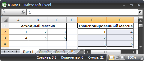
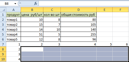
- First, we need to select the data range that will be used to transpose the table. You just need to select the area on the contrary. For example, in this example we have 4 columns and 6 rows. Therefore, it is necessary to select an area with opposite characteristics: 6 columns and 4 rows. The picture shows it very well.

- After that, we immediately begin to fill in this cell. It is important not to accidentally remove the selection. Therefore, you must specify the formula directly in the formula bar.
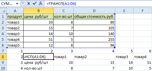
- Next, press the key combination Ctrl + Shift + Enter. Remember that this is an array formula, since we are working with a large set of data at once, which will be transferred to another large set of cells.
After we enter the data, we press the Enter key, after which we get the following result.
We see that the formula was not transferred to the new table. Formatting was also lost. Poeto
All this will have to be done manually. In addition, remember that this table is related to the original one. Therefore, as soon as some information is changed in the original range, these adjustments are automatically made to the transposed table.
Therefore, this method is well suited in cases where you need to ensure that the transposed table is linked to the original one. If you use a special insert, this possibility will no longer be.
summary table
This is a fundamentally new method, which makes it possible not only to transpose the table, but also to carry out a huge number of actions. True, the transposition mechanism will be somewhat different compared to the previous methods. The sequence of actions is as follows:
- Let’s make a pivot table. To do this, you need to select the table that we need to transpose. After that, go to the “Insert” item and look for “Pivot Table” there. A dialog box like the one in this screenshot will appear.
- Here you can reassign the range from which it will be made, as well as make a number of other settings. We are now primarily interested in the place of the pivot table – on a new sheet.
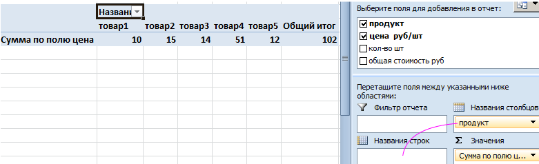
- After that, the layout of the pivot table will be automatically created. It is necessary to mark in it those items that we will use, and then they must be moved to the correct place. In our case, we need to move the “Product” item to “Column Names”, and “Price per Piece” to “Values”.
- After that, the pivot table will be finally created. An additional bonus is the automatic calculation of the final value.
- You can change other settings as well. For example, uncheck the item “Price per piece” and check the item “Total cost”. As a result, we will have a table containing information about how much the products cost. This transposition method is much more functional than the others. Let’s describe some of the benefits of pivot tables:


- Automation. With the help of pivot tables, you can summarize data automatically, as well as change the position of columns and columns arbitrarily. To do this, you do not need to perform any additional steps.
- Interactivity. The user can change the structure of information as many times as he needs to perform his tasks. For example, you can change the order of columns, as well as group data in an arbitrary way. This can be done as many times as the user needs. And it literally takes less than a minute.
- Easy to format data. It is very easy to arrange a pivot table in the way a person wants. To do this, just make a few mouse clicks.
- Getting values. The overwhelming number of formulas that are used to create reports are located in the direct accessibility of a person and are easy to integrate into a pivot table. These are data such as summation, getting the arithmetic mean, determining the number of cells, multiplying, finding the largest and smallest values in the specified sample.
- Ability to create summary charts. If PivotTables are recalculated, their associated charts are automatically updated. It is possible to create as many charts as you need. All of them can be changed for a specific task and they will not be interconnected.
- Ability to filter data.
- It is possible to build a pivot table based on more than one set of source information. Therefore, their functionality will become even greater.
True, when using pivot tables, the following restrictions must be taken into account:
- Not all information can be used to generate pivot tables. Before they can be used for this purpose, the cells must be normalized. In simple words, get it right. Mandatory requirements: presence of a header line, fullness of all lines, equality of data formats.
- The data is updated semi-automatically. To get new information in the pivot table, you must click on a special button.
- Pivot tables take up a lot of space. This may lead to some disruption of the computer. Also, the file will be difficult to send by E-mail because of this.
Also, after creating a pivot table, the user does not have the ability to add new information.