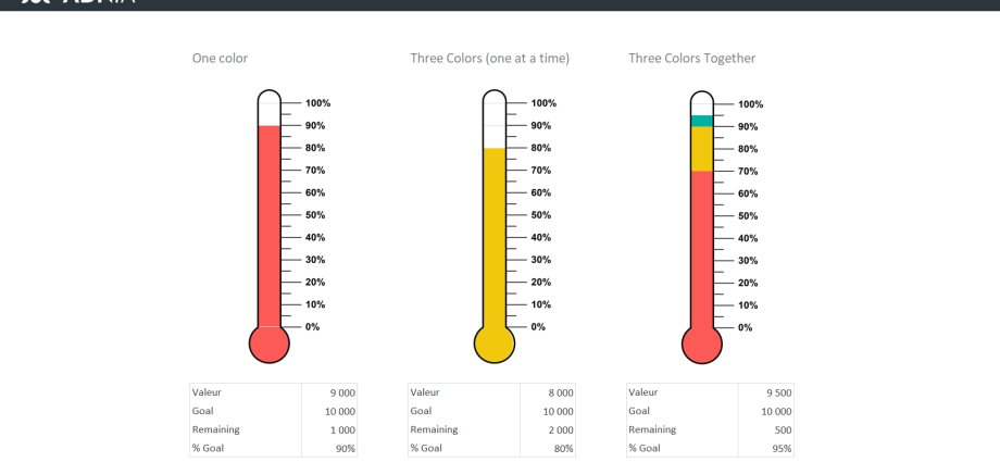
In this example, we’ll show you how to create a thermometer chart in Excel. The thermometer diagram illustrates the level of achievement of the goal.
To create a thermometer chart, follow these steps:
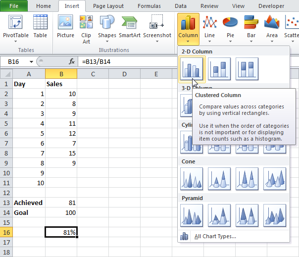
- Highlight a cell B16 (this cell must not touch other cells containing data).
- On the Advanced tab Insert (Insert) click the button Insert histogram (Column) and select Histogram with grouping (Clustered Column).
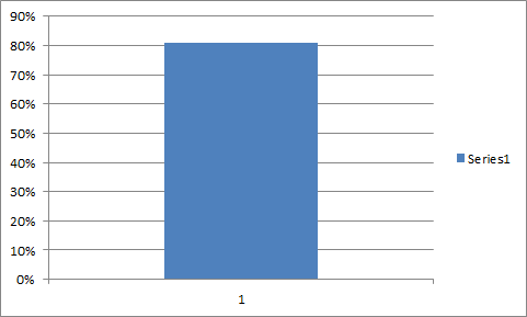
Result:
Next, set up the created chart:
- Click on the Legend located on the right side of the diagram and press the key on the keyboard Delete.
- Change the chart width.
- Right-click on the chart column, in the context menu select Data series format (Format Data Series) and for the parameter Side clearance (Gap Width) set to 0%.
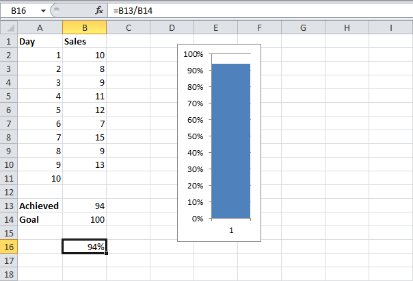
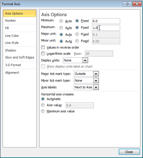
- Right-click on the percentage scale on the chart, in the context menu select Axis Format (Format Axis), set the minimum values to 0 and maximum equal to 1.

- Press Close (Close).
Result: