SUMIF function in Excel and sum by multiple conditions

Excel is an incredibly functional program. Even the built-in feature set is enough to complete almost any task. And besides the standard ones, familiar to many, there are also those that few people have heard of. But at the same time, they do not cease to be useful. They have a narrower specialization, and there is not always a need for them. But if you know about them, then at a critical moment they can be very useful.

Today we will talk about one of such functions − SUMMESLIMN.

If the user is faced with the task of summing up several values, focusing on certain criteria, then it is necessary to use the function SUMMESLIMN. The formula that uses this function takes these conditions as arguments, then sums the values ​​that meet them, and then the found value is entered into the cell in which it is written. 

SUMIFS Function Detailed Description

Before considering the function SUMMESLIMN, you must first understand what a simpler version of it is – SUMMESLI, since it is on it that the function we are considering is based. Each of us is probably already familiar with two functions that are often used – SUM (carries out the summation of values) and IF (tests a value against a specified condition).

If you combine them, you get another function – SUMMESLI, which checks the data against user-specified criteria and sums only those numbers that meet those criteria. If we talk about the English version of Excel, then this function is called SUMIF. In simple words, the -language name is a direct translation of the English-language one. This function can be used for a variety of purposes. In particular, it can be used as an alternative VPR, that is, write down

The main difference between the function SUMMESLIMN  from the usual function SUMMESLI is that several criteria are used. Its syntax is quite complex at first glance, but upon closer examination, it turns out that the logic of this function is very simple. First you need to select the range where the data will be checked, and then set the conditions for compliance with which the analysis will be performed. And such an operation can be performed for a fairly large number of conditions.

The syntax itself is:

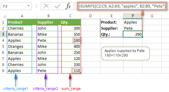
SUMIFS(sum_range, condition_range1, condition1, [condition_range2, condition2], …)

In suitable places it is necessary to put arrays of cells suitable in a particular case. 

Let’s look at the arguments in more detail:

1. Sum_range. This argument, as well as the range of condition 1 and condition 1, is required. It is a set of cells that need to be summed.
2. Condition_range1. This is the range where the condition will be checked. It is paired with the next argument – Condition1. The summation of values ​​corresponding to the criterion is carried out within the cells specified in the previous argument.
3. Condition1. This argument specifies the criteria to be checked against. It can be set, for example, in this way: “> 32”.
4. Condition range 2, Condition 2… Here, the following conditions are set in the same way. If more than a few conditions need to be specified, then the Condition Range 3 and Condition 3 arguments are added. The syntax is the same for the following arguments.

The function allows maximum processing of up to 127 pairs of conditions and ranges. 

You can use it in several areas at once (we will give just a few, the list is actually even longer):

1. Accounting. For example, it is good to use the function SUMMESLIMN to create summary reports, by quarter for spending over a certain amount, for example. Or create a report on one product from a certain price category.
2. Sales management. Here also the function can be very useful. For example, we are faced with the task of summing up only the cost of goods that were sold to a certain customer at a certain time. And in such a situation, the function SUMMESLIMN can be very helpful.
3. Education. We will give more practical examples from this area today. In particular, you can use it to get a summary of student grades. You can choose for a single subject or for individual grades. A person can immediately set several criteria by which the assessment will be selected, which is very convenient and can save a lot of time.

As you can see, the range of applications for this function is very wide. But this is not its only merit. Let’s take a look at a few more benefits that this feature has:

1. Ability to set multiple criteria. Why is this an advantage? You can use the normal function SUMMESLI! And all because it is convenient. There is no need to carry out separate calculations for each of the criteria. All actions can be programmed in advance, even before. how the data table will be formed. This is a great time saver.
2. Automation. The modern age is the age of automation. Only the person who knows how to properly automate his work can earn a lot. That is why the ability to master Excel and the function SUMMESLIMN in particular, is so important for any person who wants to build a career. Knowing one function allows you to perform several actions at once, as one. And here we move on to the next benefit of this feature.
3. Saving time. Just due to the fact that one function performs several tasks at once.
4. Simplicity. Despite the fact that the syntax is quite heavy at first glance due to its bulkiness, in fact, the logic of this function is very simple. First, a range of data is selected, then a range of values, which will be checked for compliance with a certain condition. And of course, the condition itself must also be specified. And so several times. In fact, this function is based on only one logical construct, which makes it simpler than the well-known VPR despite the fact that it can be used for the same purposes, also taking into account a larger number of criteria. 

Features of using the SUMIFS function

There are several features of using this function that you need to pay attention to. First of all, this function ignores ranges with text strings or nulls, since these data types cannot be added together in an arithmetic pattern, only concatenated like strings. This function cannot do this. You also need to pay attention to the following conditions:

1. You can use these types of values ​​as conditions for selecting cells to further add the values ​​contained in them: numeric values, boolean expressions, cell references, and so on. 
2. If text, logical expressions or mathematical signs are being checked, then such criteria are specified through quotes.
3. Cannot use terms longer than 255 characters.
4. It is possible to use approximate criteria for selecting values ​​using wildcards. The question mark is used to replace a single character, and the multiplication sign (asterisk) is needed to replace multiple characters. 
5. Boolean values ​​that are in the summation range are automatically converted to numeric values ​​according to their type. Thus, the value “TRUE” turns into one, and “FALSE” – into zero. 
6. If a #VALUE! error appears in a cell, it means that the number of cells in the condition and summation ranges is different. You need to make sure that the sizes of these arguments are the same. 

Examples of using the SUMIFS function

Function SUMMESLIMN not as complicated as it seems at first glance, it turns out. But for more clarity, let’s look at some practical examples of how you can use the function SUMMESLIMN. This will make it much easier to delve into the topic.

Condition summation dynamic range

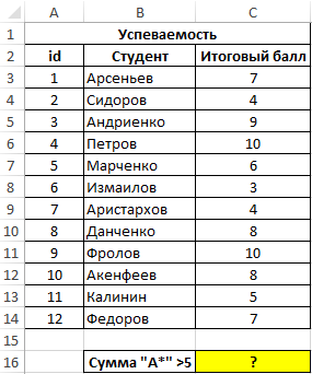
So let’s start with the first example. Let’s say we have a table that contains information about how students cope with the curriculum in a particular subject. There is a set of grades, performance is assessed on a 10-point scale. The task is to find the grade for the exam of those students whose last name begins with the letter A, and their minimum score is 5.

The table looks like this.

In order for us to calculate the total score based on the criteria described above, we need to apply the following formula.

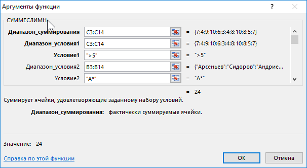
Let’s describe the arguments in more detail:

1. C3:C14 is our summation range. In our case, it coincides with the condition range. From it will be selected points used to calculate the amount, but only those that fall under our criteria.
2. “>5” is our first condition.
3. B3:B14 is the second summation range that is processed to match the second criterion. We see that there is no coincidence with the summation range. From this we conclude that the range of summation and the range of the condition may or may not be identical. 
4. “A*” is the second range, which specifies the selection of marks only for those students whose last name begins with A. In our case, an asterisk means any number of characters. 

After calculations, we get the following table.

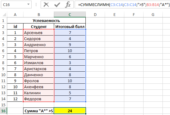
As you can see, the formula summed up the values ​​based on the dynamic range and based on the conditions specified by the user.

Selective summation by condition in Excel

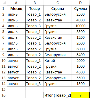
Now suppose we want to get information about what goods were shipped to which countries during the last quarter. After that, find the total revenue from shipments for July and August.

The table itself looks like this. 

To determine the final result, we need such a formula.

=(СУММЕСЛИМН(D2:D14;A2:A14;»=июнь»;B2:B14;»Товар_2″;C2:C14;»Казахстан»)+(СУММЕСЛИМН(D2:D14;A2:A14;»=август»;B2:B14;»Товар_2″;C2:C14;»Казахстан»)))

As a result of the calculations carried out by this formula, we get the following result.

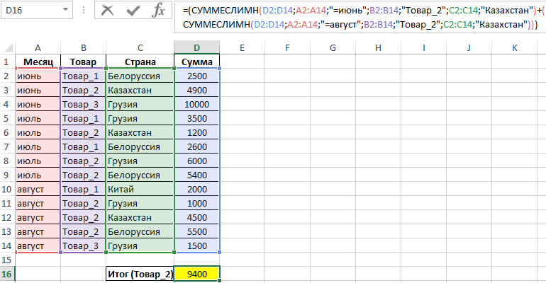
Attention! This formula looks pretty big even though we only used two criteria. If the data range is the same, then you can significantly reduce the length of the formula, as shown below.

SUMIFS function to sum values ​​across multiple conditions

Now let’s give another example to illustrate. In this case, the table remains the same as in the previous case. 

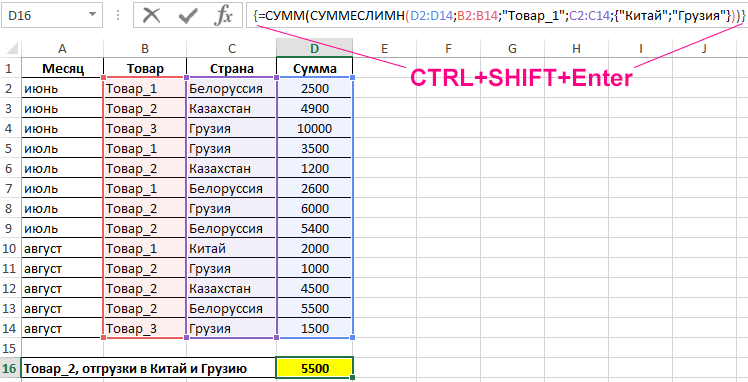
We use the following formula (but we write it as an array formula, that is, we enter it through the key combination CTRL + SHIFT + ENTER).

=СУММ(СУММЕСЛИМН(D2:D14;B2:B14;»Товар_1″;C2:C14;{«Китай»;»Грузия»}))

After the function SUMMESLIMN will sum the array of values ​​based on the criteria specified in the formula (that is, the countries of China and Georgia), the resulting array is summed by the usual function SUM, which is written as an array formula.

If the conditions were passed as an array constant for more than one pair, then the formula will give an incorrect result.

Now let’s take a look at the table containing the totals.

As you can see, we have succeeded. You will definitely succeed too. Great success in this field. This is a very simple function that a person who has just set foot on the path of learning Excel can understand. And we already know that the function SUMMESLIMN allows you to be effective in any field of activity, from accounting to even education. Even if you are building a career in any other area that has not been described above, this feature will still help you earn money. This is why she is valuable.

Most importantly, it allows you to save time, which is, unfortunately, a limited resource. It would seem that there are a couple of seconds to apply two functions, but when you have to perform a huge number of repetitive operations, then these seconds add up to hours that could be spent on something else. So we recommend that you practice using this feature. Moreover, it is incredibly simple.