Subtracting numbers in Excel

Among all arithmetic operations, four main ones can be distinguished: addition, multiplication, division and subtraction. The latter will be discussed in this article. Let’s look at what methods you can perform this action in Excel.

subtraction procedure

Subtraction in Excel can involve both specific numbers and cells containing numerical values.

The action itself can be performed using a formula that begins with the sign “equals” (“=”). Then, according to the laws of arithmetic, we write minuend, after which I put a sign “minus” (“-“) and at the end indicate subtrahend. In complex formulas, there can be several subtrahends, and in this case, they follow, and between them is put “-“. Thus, we get the result in the form of a difference of numbers.

For more clarity, let’s look at how to perform subtraction using specific examples below.

Example 1: Difference of Specific Numbers

Let’s say we need to find the difference between specific numbers: 396 and 264. You can perform the subtraction using a simple formula:

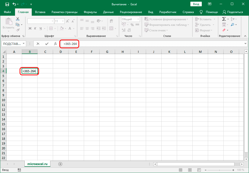
1. We pass to a free cell of the table in which we plan to make the necessary calculations. We print a sign in it “=”, after which we write the expression: =365-264.
2. After the formula is typed, press the key Enter and we get the required result.

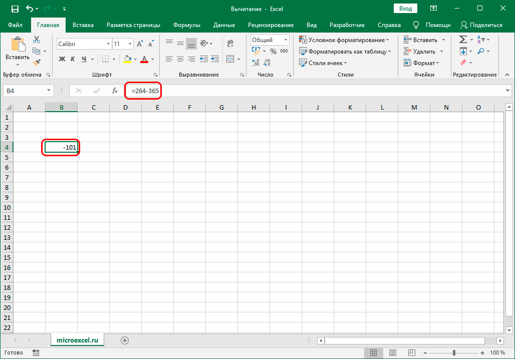
Note: Of course, the Excel program can work with negative numbers, therefore, subtraction can be performed in reverse order. In this case, the formula looks like this: =264-365.

Example 2: subtracting a number from a cell

Now that we have covered the principle and the simplest example of subtraction in Excel, let’s see how to subtract a specific number from a cell.

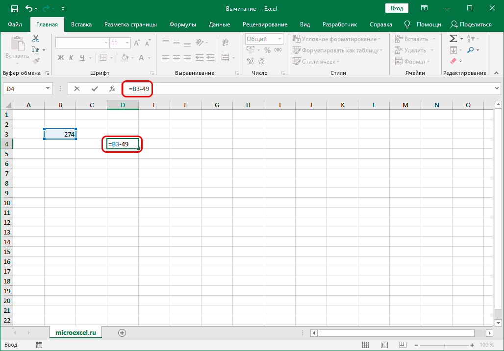
1. As in the first method, first select a free cell where we want to display the result of the calculation. In it:
   • we write a sign “=”.
   • specify the address of the cell in which the minuend is located. You can do this manually by entering the coordinates using the keys on the keyboard. Or you can select the desired cell by clicking on it with the left mouse button.
   • add a subtraction sign to the formula (“-“).
   • write the subtrahend (if there are several subtrahends, add them through the symbol “-“).
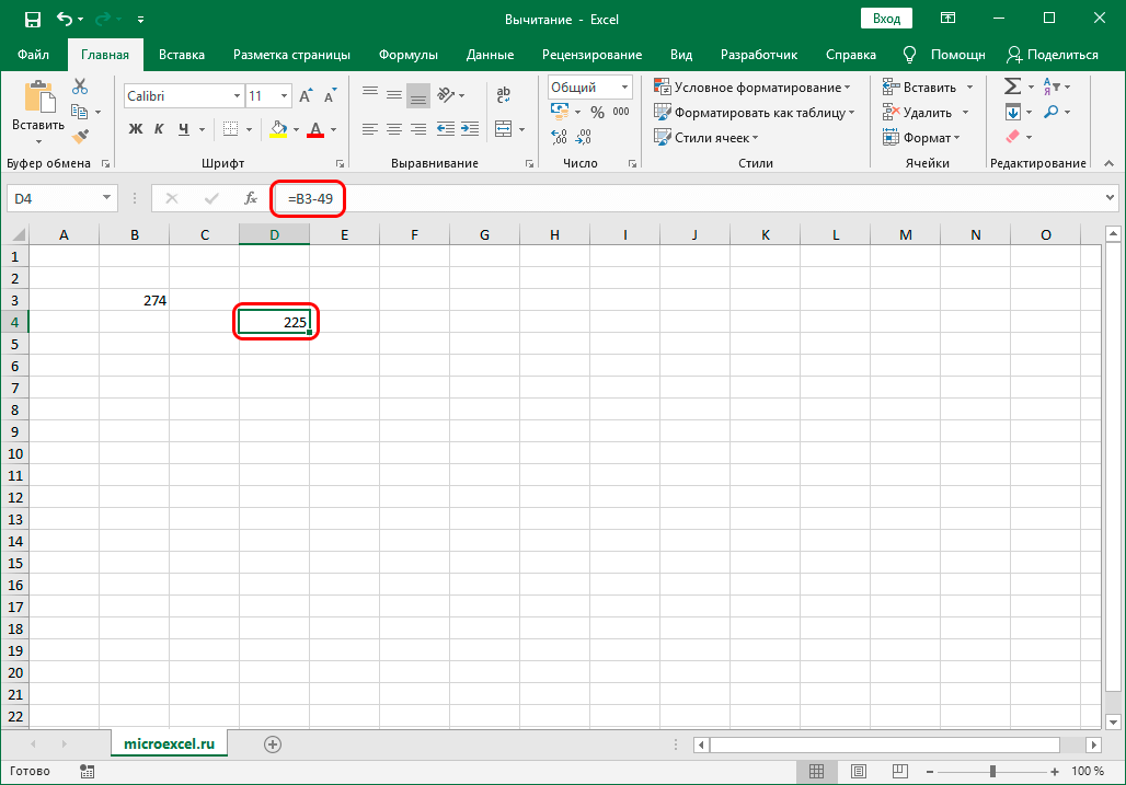
2. After pressing the key Enter, we get the result in the selected cell.

Note: this example also works in reverse order, i.e. when the minuend is a specific number, and the subtrahend is the numeric value in the cell.

Example 3: difference between numbers in cells

Since in Excel we, first of all, work with the values ​​in the cells, then the subtraction, most often, has to be carried out between the numeric data in them. The steps are almost identical to those described above.

1. We get up in the resulting cell, after which:
   • put a symbol “=”.
   • similarly to example 2, we indicate the cell containing the reduced.
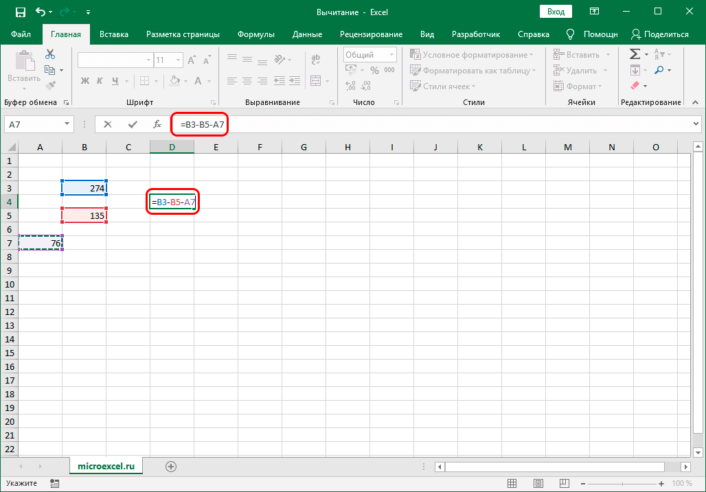
   • in the same way, add a cell with a subtrahend to the formula, not forgetting to add a sign in front of its address “minus”.
   • if there are several to be subtracted, add them in a row with a sign “-“ ahead.
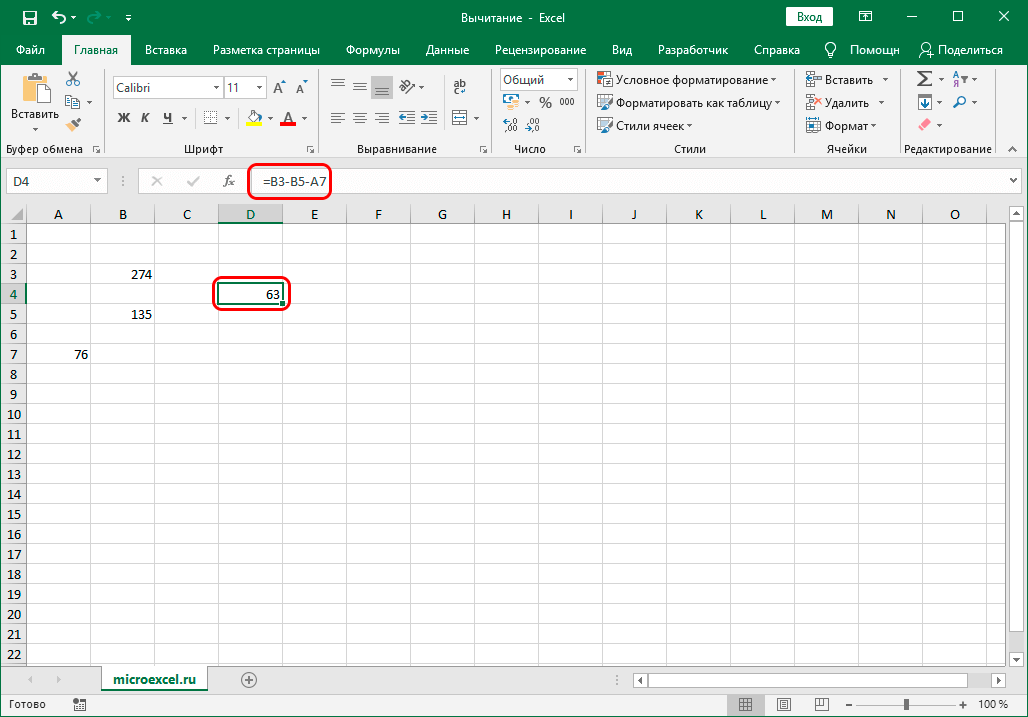
2. By pressing the key Enter, we will see the result in the formula cell.

Example 4: Subtracting one column from another

Tables, as we know, contain data both horizontally (columns) and vertically (rows). And quite often it is required to find the difference between the numerical data contained in different columns (two or more). Moreover, it is desirable to automate this process so as not to spend a lot of time on this task.

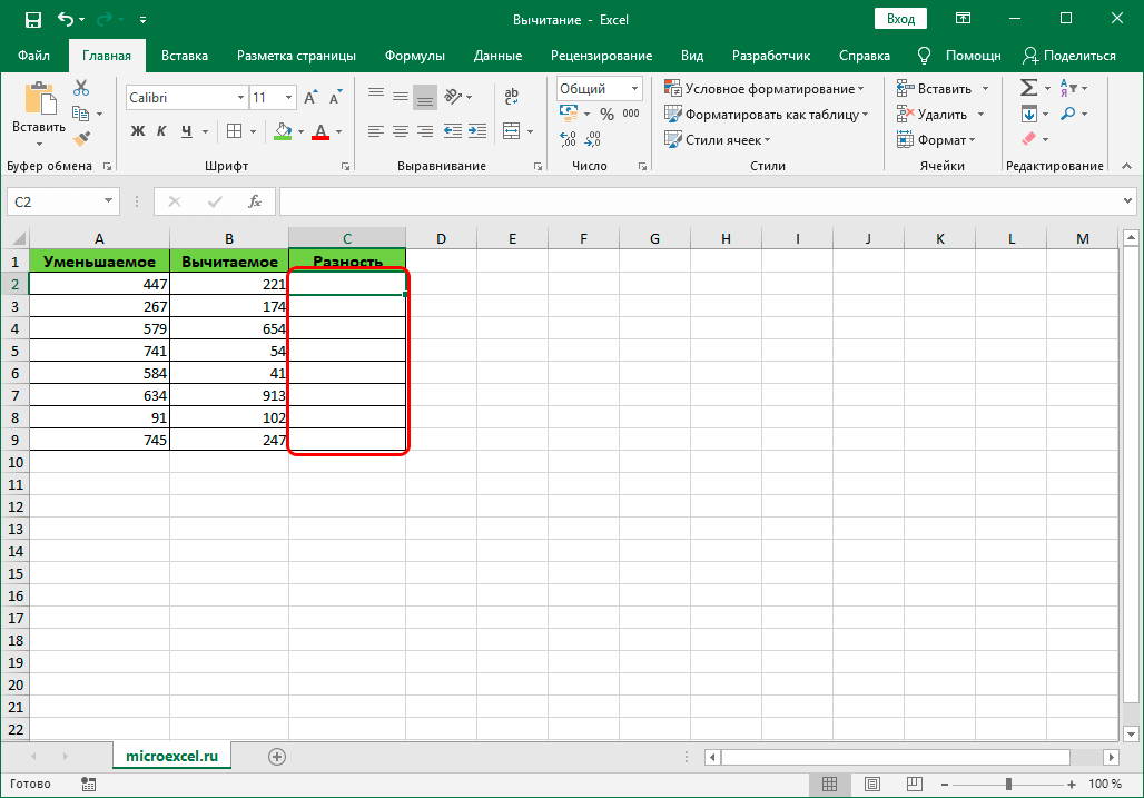
The program provides the user with such an opportunity, and here is how it can be implemented:

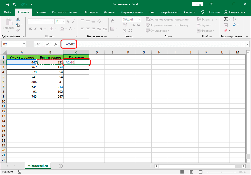
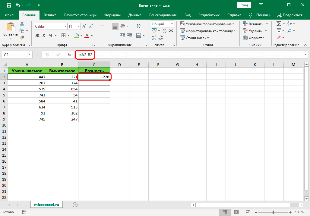
1. Go to the first cell of the column in which we plan to make calculations. We write the subtraction formula, indicating the addresses of the cells that contain the minuend and the subtrahend. In our case, the expression looks like this: =С2-B2.
2. Press the key Enter and get the difference of numbers.
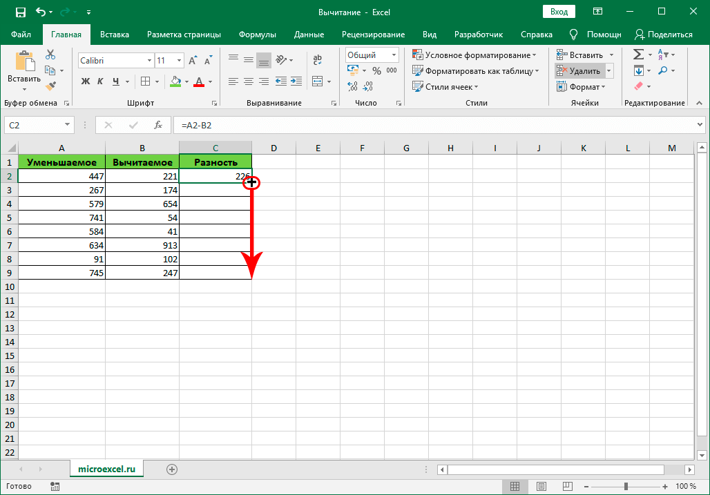
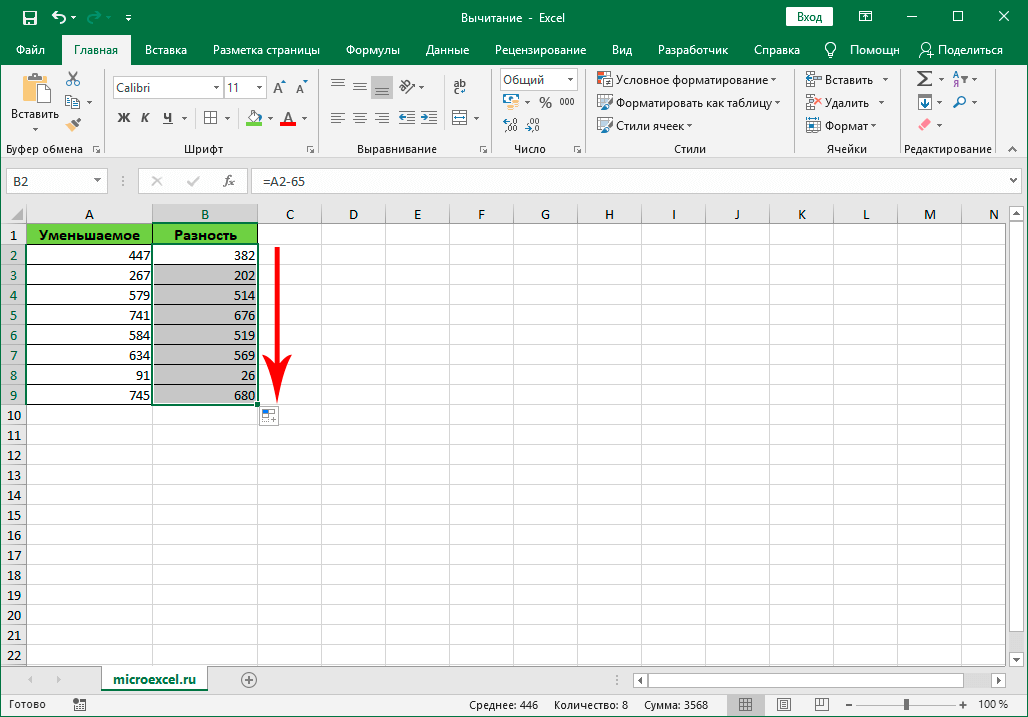
3. It remains only to automatically perform the subtraction for the remaining cells of the column with the results. To do this, move the mouse pointer to the lower right corner of the cell with the formula, and after the fill marker appears in the form of a black plus sign, hold down the left mouse button and drag it to the end of the column.
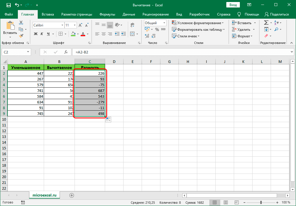
4. As soon as we release the mouse button, the column cells will be filled with the results of the subtraction.

Example 5: Subtracting a specific number from a column

In some cases, you want to subtract the same specific number from all cells in a column.

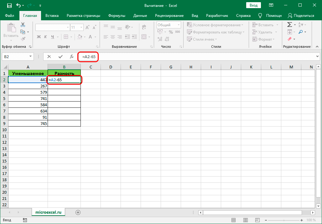
This number can simply be specified in the formula. Let’s say we want to subtract a number from the first column of our table 65.

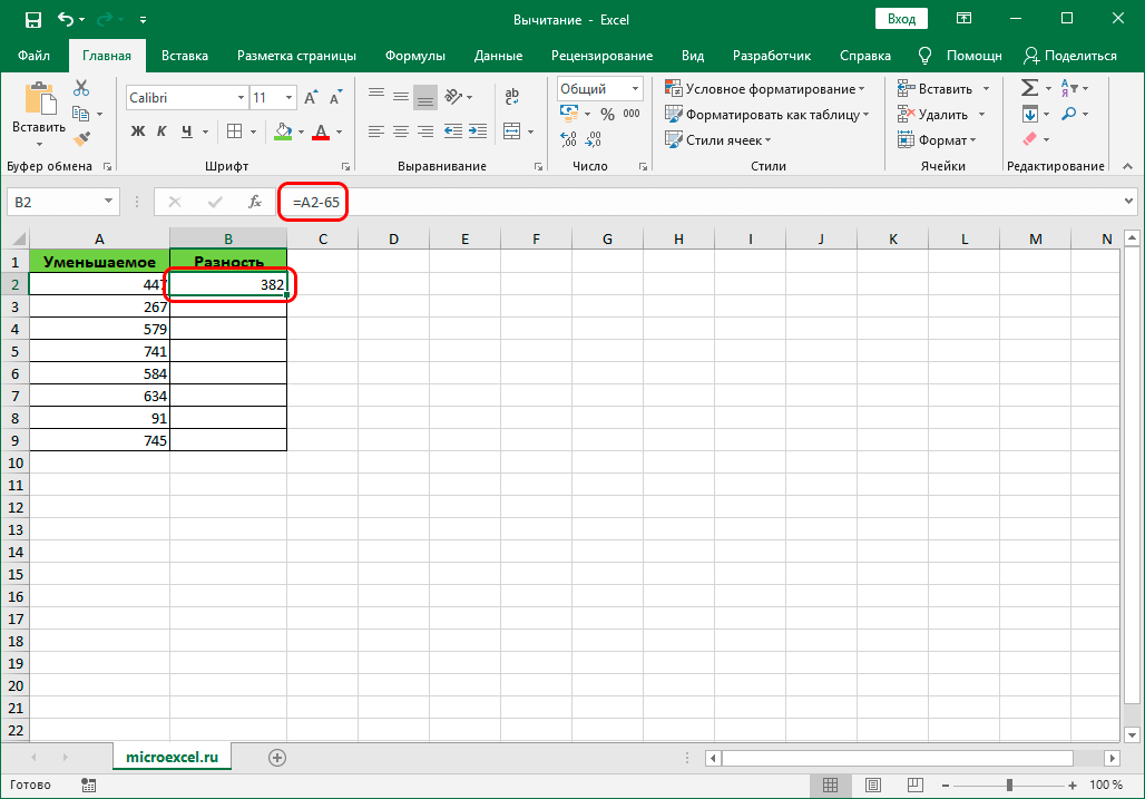
1. We write the subtraction formula in the topmost cell of the resulting column. In our case, it looks like this: =A2-65.
2. After clicking Enter the difference will be displayed in the selected cell.
3. Using the fill handle, we drag the formula to other cells in the column to get similar results in them.

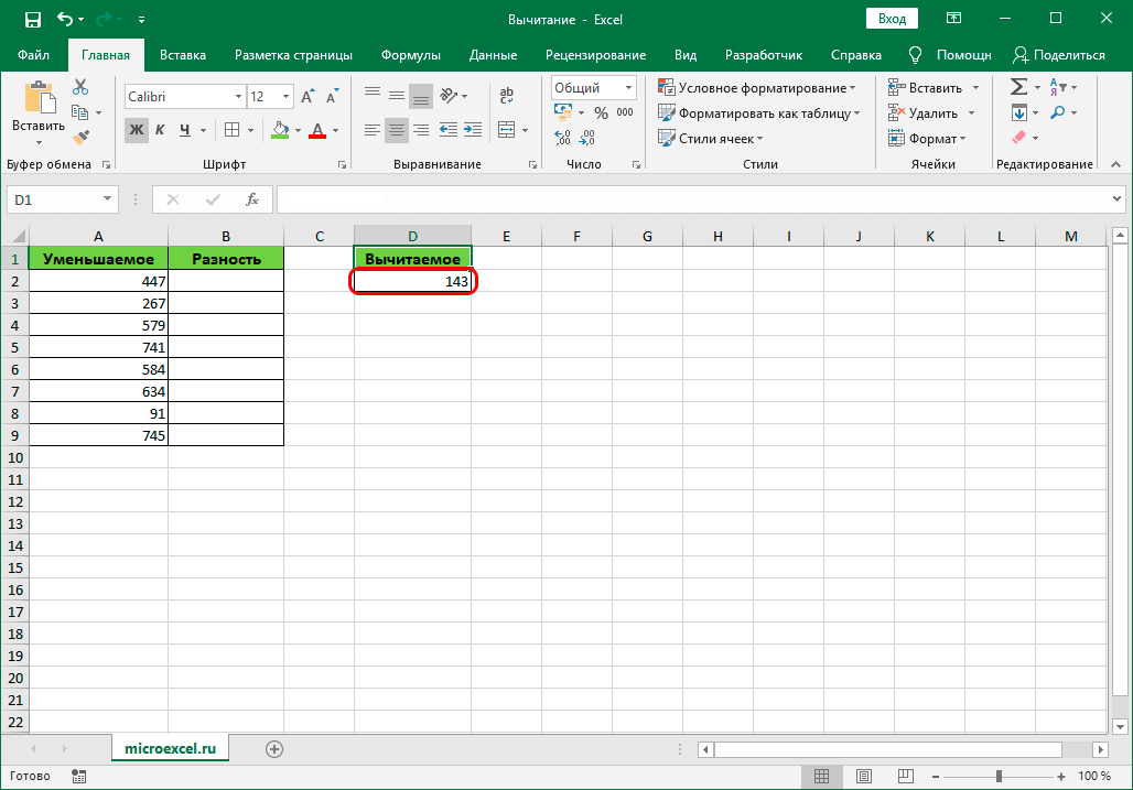
Now let’s suppose that we want subtract a specific number from all cells of the column, but it will not only be indicated in the formula, but will also be written in a specific cell.

The undoubted advantage of this method is that if we want to change this number, it will be enough for us to change it in one place – in the cell containing it (in our case, D2).

The algorithm of actions in this case is as follows:

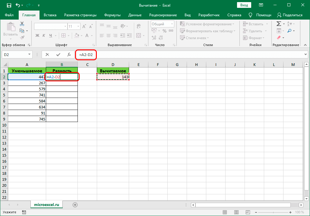
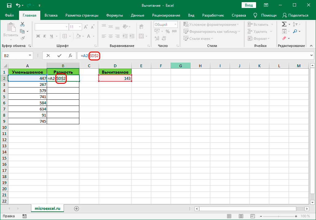
1. Go to the topmost cell of the column for calculations. We write in it the usual subtraction formula between two cells.
2. When the formula is ready, do not rush to press the key Enter. In order to fix the address of the cell with the subtrahend when stretching the formula, you need to insert symbols opposite its coordinates “$” (in other words, make the cell address absolute, since by default the links in the program are relative). You can do this manually by entering the necessary characters in the formula, or, when editing it, move the cursor to the address of the cell with the subtrahend and press the key once F4. As a result, the formula (in our case) should look like this:
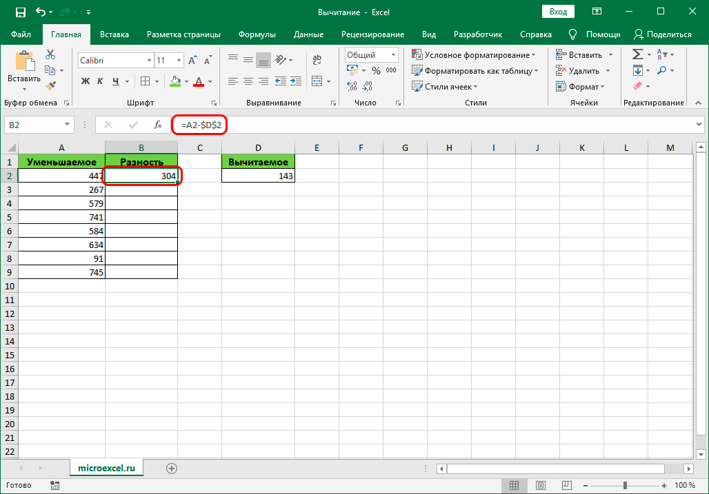
3. After the formula is completely ready, click Enter to get a result.
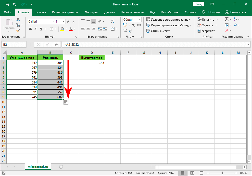
4. Using the fill marker, we perform similar calculations in the remaining cells of the column.

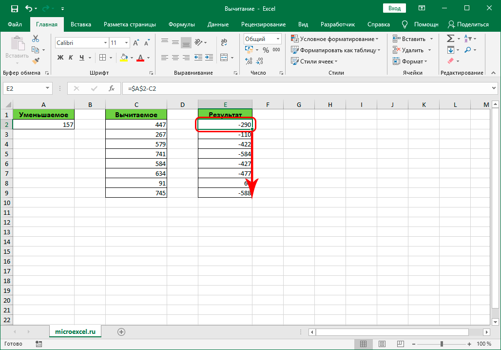
Note: The above example can be considered in reverse order. Those. subtract from the same cell data from another column.

Conclusion

Thus, Excel provides the user with a great variety of actions, thanks to which such an arithmetic operation as subtraction can be performed in a variety of ways, which, of course, allows you to cope with a task of any complexity.