


Method 1. Formulas
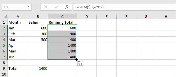
Let’s start, for warming up, with the simplest option – formulas. If we have a small table sorted by date as input, then to calculate the running total in a separate column, we need an elementary formula:

The main feature here is the tricky fixing of the range inside the SUM function – the reference to the beginning of the range is made absolute (with dollar signs), and to the end – relative (without dollars). Accordingly, when copying the formula down to the entire column, we get an expanding range, the sum of which we calculate.
The disadvantages of this approach are obvious:
- The table must be sorted by date.
- When adding new rows with data, the formula will have to be extended manually.
Method 2. Pivot table
This method is a little more complicated, but much more pleasant. And to exacerbate, let’s consider a more serious problem – a table of 2000 rows of data, where there is no sorting by the date column, but there are repetitions (i.e. we can sell several times on the same day):

We convert our original table into a “smart” (dynamic) keyboard shortcut Ctrl+T or team Home – Format as a table (Home — Format as Table), and then we build a pivot table on it with the command Insert – PivotTable (Insert — Pivot Table). We put the date in the rows area in the summary, and the number of goods sold in the values area:

Please note that if you have a not quite old version of Excel, then the dates are automatically grouped by years, quarters and months. If you need a different grouping (or do not need it at all), then you can fix it by right-clicking on any date and selecting commands Group / Ungroup (Group / Ungroup).
If you want to see both the resulting totals by periods and the running total in a separate column, then it makes sense to throw the field into the value area Sold again to get a duplicate of the field – in it we will turn on the display of running totals. To do this, right-click on the field and select the command Additional Calculations – Cumulative Total (Show Values as — Running Totals):

There you can also select the option of growing totals as a percentage, and in the next window you need to select the field for which the accumulation will go – in our case, this is the date field:

The advantages of this approach:
- A large amount of data is quickly read.
- No formulas need to be entered manually.
- When changing in the source data, it is enough to update the summary with the right mouse button or with the Data – Refresh All command.
The disadvantages follow from the fact that this is a summary, which means that you can’t do whatever you want in it (insert lines, write formulas, build any diagrams, etc.) will no longer work.
Method 3: Power Query
Let’s load our “smart” table with source data into the Power Query query editor using the command Data – From Table/Range (Data — From Table/Range). In the latest versions of Excel, by the way, it was renamed – now it is called With leaves (From Sheet):

Then we will perform the following steps:
1. Sort the table in ascending order by the date column with the command Sort ascending in the filter drop-down list in the table header.
2. A little later, to calculate the running total, we need an auxiliary column with the ordinal row number. Let’s add it with the command Add Column – Index Column – From 1 (Add column — Index column — From 1).
3. Also, to calculate the running total, we need a reference to the column Sold, where our summarized data lies. In Power Query, columns are also called lists (list) and to get a link to it, right-click on the column header and select the command Detailing (Show detail). The expression we need will appear in the formula bar, consisting of the name of the previous step #”Index added”, from where we take the table and the column name [Sales] from this table in square brackets:

Copy this expression to the clipboard for further use.
4. Delete unnecessary more last step Sold and add instead a calculated column for calculating the running total with the command Adding a Column – Custom Column (Add column — Custom column). The formula we need will look like this:

Here the function List.Range takes the original list (column [Sales]) and extracts elements from it, starting from the first (in the formula, this is 0, since numbering in Power Query starts from zero). The number of elements to retrieve is the row number we take from the column [Index]. So this function for the first row only returns one first cell of the column Sold. For the second line – already the first two cells, for the third – the first three, etc.
Well, then the function List.Sum sums the extracted values and we get in each row the sum of all previous elements, i.e. cumulative total:

It remains to delete the Index column that we no longer need and upload the results back to Excel with the Home – Close & Load to command.
The problem is solved.
Fast and Furious
In principle, this could have been stopped, but there is a small fly in the ointment – the request we created works at the speed of a turtle. For example, on my not the weakest PC, a table of only 2000 rows is processed in 17 seconds. What if there is more data?
To speed up, you can use buffering using the special List.Buffer function, which loads the list (list) given to it as an argument into RAM, which greatly speeds up access to it in the future. In our case, it makes sense to buffer the #”Added index”[Sold] list, which Power Query has to access when calculating the running total in each row of our 2000-row table.
To do this, in the Power Query editor on the Main tab, click the Advanced Editor button (Home – Advanced Editor) to open the source code of our query in the M language built into Power Query:

And then add a line with a variable there MyList, the value of which is returned by the buffering function, and at the next step we replace the call to the list with this variable:

After making these changes, our query will become significantly faster and will cope with a 2000-row table in just 0.3 seconds!
Another thing, right? 🙂
- Pareto chart (80/20) and how to build it in Excel
- Keyword search in text and query buffering in Power Query