


Over time, your Excel workbook has more and more rows of data that become more and more difficult to work with. Therefore, there is an urgent need to hide some of the filled lines and thereby unload the worksheet. Hidden rows in Excel do not clutter up the sheet with unnecessary information and at the same time participate in all calculations. In this lesson, you will learn how to hide and show hidden rows and columns, as well as move them if necessary.
Move rows and columns in Excel
Sometimes it becomes necessary to move a column or row to reorganize a sheet. In the following example, we will learn how to move a column, but you can move a row in exactly the same way.
- Select the column you want to move by clicking on its header. Then press the Cut command on the Home tab or the keyboard shortcut Ctrl+X.
- Select the column to the right of the intended insertion point. For example, if you want to place a floating column between columns B and C, select column C.
- On the Home tab, from the drop-down menu of the Paste command, select Paste Cut Cells.
- The column will be moved to the selected location.
You can use the Cut and Paste commands by right-clicking and selecting the necessary commands from the context menu.
Hiding rows and columns in Excel
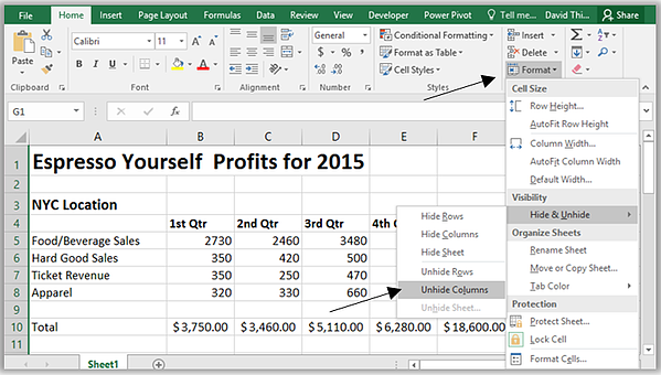
Sometimes it becomes necessary to hide some rows or columns, for example, to compare them if they are located far from each other. Excel allows you to hide rows and columns as needed. In the following example, we will hide columns C and D in order to compare A, B and E. You can hide rows in the same way.
- Select the columns you want to hide. Then right-click on the selected range and select Hide from the context menu.
- The selected columns will be hidden. The green line shows the location of the hidden columns.
- To show hidden columns, select the columns to the left and right of the hidden ones (in other words, on either side of the hidden ones). In our example, these are columns B and E.
- Right-click on the selected range, then select Show from the context menu. The hidden columns will reappear on the screen.