


Contents
Данное руководство расскажет, как в Excel создать линейчатую диаграмму со значениями, автоматически отсортированными по убыванию или по возрастанию, как создать линейчатую диаграмму с отрицательными значениями, как настраивать ширину полос линейчатой диаграммы и многое другое.
Bar charts, along with pie charts, are among the most popular charts. It is not difficult to build a bar chart, but it is even easier to understand. What is the best data to use a bar chart for? For any numerical data that needs to be compared: numbers, percentages, temperatures, frequencies, and other measurements. In general, a bar chart is suitable for comparing the individual values of several categories of data. A special kind of bar chart, the Gantt chart, is often used in project management applications.
In this tutorial, we will cover the following questions regarding bar charts in Excel:
Линейчатые диаграммы в Excel – основы
Bar chart is a graph showing different categories of data as rectangular bars (bars) whose lengths are proportional to the values of the data items they represent. Such stripes can be arranged horizontally (линейчатая диаграмма) or vertically. A vertical bar chart is a separate type of chart in Excel called bar chart.
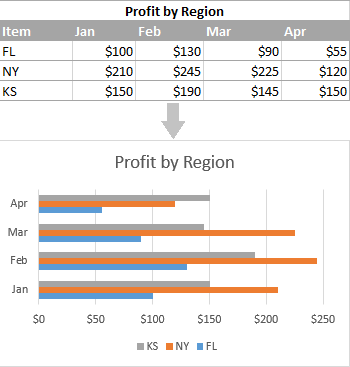
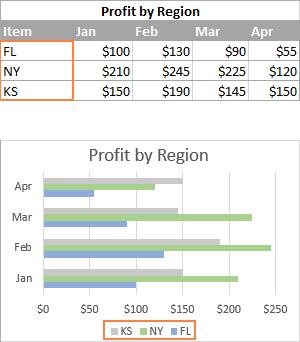
To simplify the further study of this guide and to know for sure that we understand each other correctly, let’s define the main terms that denote the elements of a bar chart in Excel. The following figure shows a standard grouped bar chart that contains 3 data series (grey, green, and blue) and 4 data categories (Jan, Feb, Mar, and Apr).
How to build a bar chart in Excel
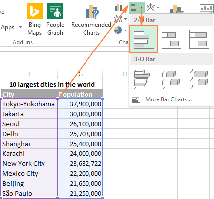
There is nothing easier than building a bar chart in Excel. First select the data you want to show in the chart, then on the tab Insert (Insert) in section Diagrams (Charts) Click the bar chart icon and select which subtype to create.
В данном примере мы создаём самую простую диаграмму – Grouped line (2-D clustered Bar):
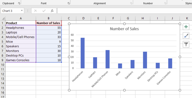
Grouped bar chart, pasted into an Excel worksheet, would look something like this:
The Excel bar chart shown in the figure above only displays one series of data because the source data contains only one column of numbers. If there are two or more columns with numbers in the source data, then the bar chart will contain several data series, colored in different colors:
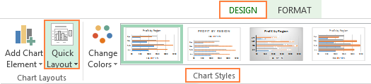
How to see all available bar chart types
To see all the bar chart types available in Excel, click the link Other bar charts (More Column Charts) and in the opened dialog box Insert a chart (Insert Chart) select one of the available chart subtypes.
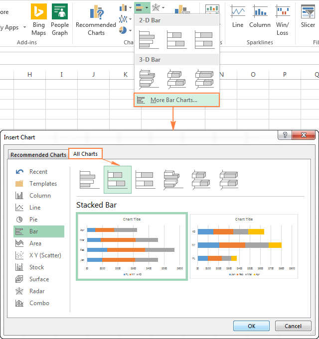
Choosing a Bar Chart Layout and Style
If you don’t like the default layout or style of a bar chart inserted into your Excel worksheet, select it to display a group of tabs on the Menu Ribbon Working with charts (ChartTools). After that, on the tab Constructor (Design) you can do the following:
- In section Chart layouts (Chart Layouts) click the button Express layout (Quick Layout) and try different ready-made bar chart layouts;
- Or experiment with bar chart styles in the section Chart styles (Chart Styles).

Типы линейчатых диаграмм в Excel
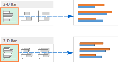
When creating a bar chart in Excel, you can select one of the following subtypes:
Grouped line
A grouped bar chart (2-D or 3-D) compares values in data categories. In a grouped bar chart, the categories are usually plotted along the vertical axis (y-axis) and the values are plotted along the horizontal axis (x-axis). A grouped 3-D bar chart does not display a third axis, but simply makes the bars of the graph appear XNUMXD.
Ruled Stacked
A stacked bar chart shows the proportions of individual elements in relation to the whole. Like the grouped bar chart, it can be either flat (2-D) or 3-D (XNUMX-D):
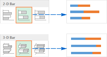
Нормированная линейчатая с накоплением
This type of bar chart is similar to the previous one, but shows the percentage of each item relative to the whole for each data category.
Cylinders, cones and pyramids
Кроме стандартных прямоугольников, для построения всех перечисленных подтипов линейчатой диаграммы можно использовать цилиндры, конусы или пирамиды. Разница только в форме фигуры, которая отображает исходные данные.
In Excel 2010 and earlier, you could create a cylinder, cone, or pyramid chart by selecting the appropriate chart type from the tab. Insert (Insert) in section Diagrams (Charts).
The Excel 2013 and Excel 2016 Menu Ribbon does not offer cylinders, cones, or pyramids. According to Microsoft, these chart types were removed because too many chart types in earlier versions of Excel made it difficult for the user to select the right type. However, the ability to use a cylinder, cone, or pyramid is also available in modern versions of Excel, although this requires a few additional steps.
How to use a cylinder, cone, or pyramid when plotting a chart in Excel 2013 and 2016
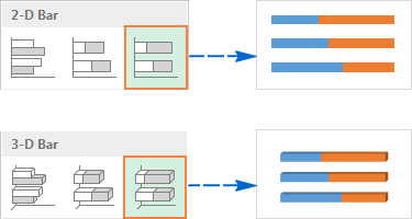
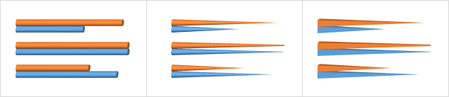
To use a cylinder, cone, or pyramid chart in Excel 2013 and 2016, create a XNUMX-D bar chart of the desired type (grouped, stacked, or normalized stacked) and then modify the shapes used to plot the series:
- Select all the bars on the chart, right-click on them and in the context menu click Data series format (Format Data Series), or simply double-click on the graph bar.
- In the panel that appears, in the section Row Options (Series Options) выберите подходящую Figure (Column shape).
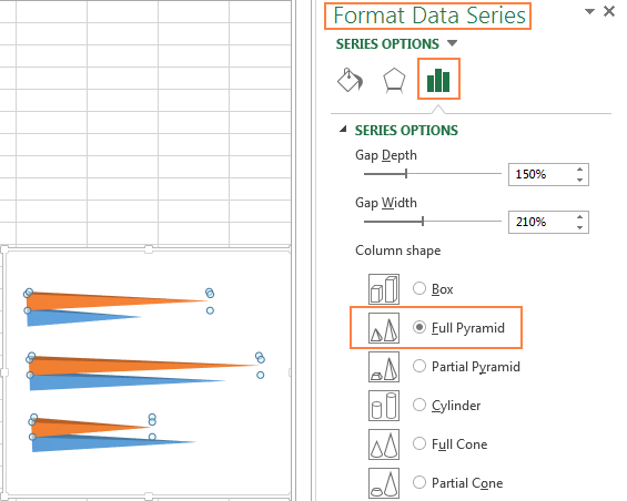
Note: Если на диаграмме построено несколько рядов данных, то описанную процедуру необходимо повторить для каждого ряда в отдельности.
Setting up bar charts in Excel
Like other types of Excel charts, bar charts provide a lot of customization for elements such as chart title, axes, data labels, and more. You can find more detailed information on the links below:
Now let’s look at some specific tricks that apply to bar charts in Excel.
Change the width of the bars and the distance between the chart bars
A bar chart created in Excel using the default settings has too much empty space between the bars. To make the stripes wider and visually closer to each other, follow these steps. In the same way, you can make the stripes narrower and increase the distance between them. In a flat 2-D chart, the bars can even overlap.
- In an Excel bar chart, right-click on any data series (bar) and from the context menu, click Data series format (Format Data Series)
- In the panel that appears, in the section Row Options (Series Options) do one of the following:
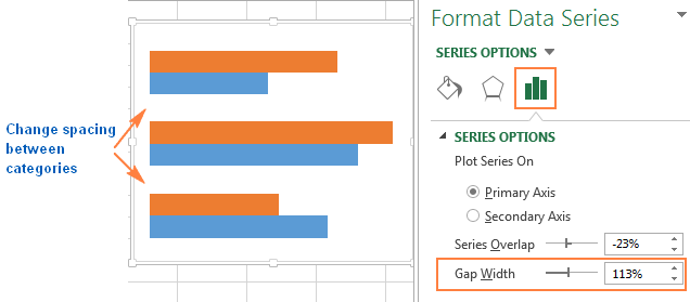
- For flatsoh or for a XNUMXD chart: чтобы изменить ширину полосы и промежуток между категориями, переместите ползунок параметра Side clearance (Gap Width) or enter a percentage value from 0 to 500 in the input field. The lower the value, the thinner the stripes and the smaller the gap between them, and vice versa.
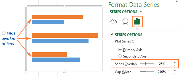
- Для плоской диаграммы: чтобы изменить зазор между рядами в одной категории, переместите ползунок параметра overlapping rows (Series Overlap) or enter a percentage value from -100 to 100 in the input field. The larger the value, the greater the overlap of the series. A negative value will result in a gap between the rows, as in the picture below:
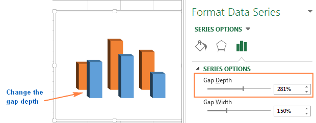
- For a 3D (XNUMX-D) chart: to change the spacing between data series, move the parameter slider Front clearance (Gap Depth) или введите значение от 0 до 500 процентов. Чем больше значение, тем больше расстояние между полосами. Изменение фронтального зазора заметно отражается в большинстве линейчатых диаграмм Excel, но лучше всего – в объёмной гистограмме, как показано на следующей картинке:
- For flatsoh or for a XNUMXD chart: чтобы изменить ширину полосы и промежуток между категориями, переместите ползунок параметра Side clearance (Gap Width) or enter a percentage value from 0 to 500 in the input field. The lower the value, the thinner the stripes and the smaller the gap between them, and vice versa.
Building a bar chart with negative values
To build a bar chart in Excel, the original values do not have to be greater than zero. In general, Excel has no problems with displaying negative values on a standard bar chart, but the appearance of the chart inserted by default on an Excel worksheet makes you think about editing layout and design.
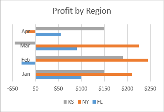
In order to somehow improve the look of the chart in the figure above, firstly, it would be nice to shift the vertical axis labels to the left so that they do not overlap with the negative value bars, and secondly, you can use other colors for negative values.
Настраиваем подписи вертикальной оси
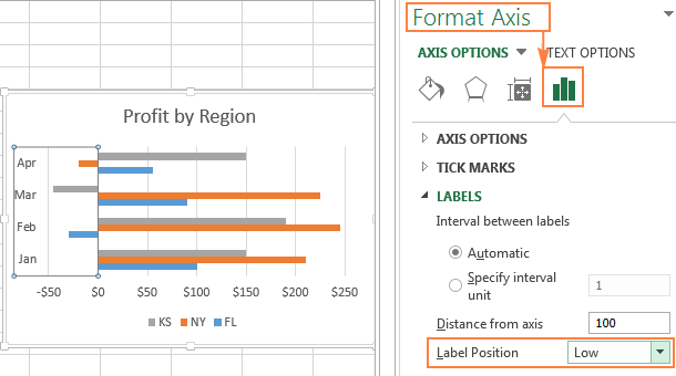
To change the appearance of the vertical axis, click on any of its labels and in the context menu, click Axis Format (Format Axis), или просто дважды кликните по подписям оси. В правой части рабочего листа появится панель.
Click the Axis parameters (Axis Options), expand the section signatures (Labels) и установите для параметра Label position (Labels Position) значение At the bottom (Low).
Меняем цвет заливки для отрицательных значений
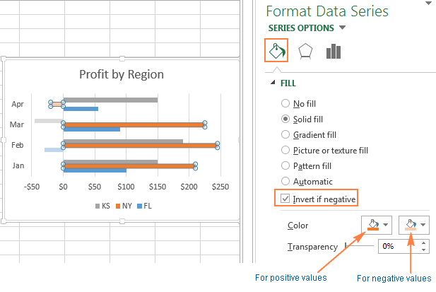
If you want to draw attention to the negative values on the chart, then this can be successfully done if the bars of negative values are painted in a different color.
Если в линейчатой диаграмме Excel построен только один ряд данных, то отрицательные значения, как это часто делается, можно окрасить в красный цвет. Если рядов данных на диаграмме несколько, то отрицательные значения в каждом из них нужно будет окрасить в свой цвет. Например, можно использовать определенные цвета для положительных значений, а для отрицательных — их более бледные оттенки.
To change the color of the negative bars, follow these steps:
- Кликните правой кнопкой мыши по любой полосе ряда данных, цвет которого нужно изменить (в нашем примере это оранжевая полоса) и в контекстном меню нажмите Data series format (Format Data Series).
- В появившейся панели на вкладке Shading and Borders (Fill & Line) tick option Inversion for numbers <0 (Invert if Negative)
- Immediately after that, two color selection boxes will appear – for positive and for negative values.
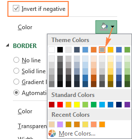
Tip: If the second color picker doesn’t appear, click on the little black arrow in the only available box so far and specify a color for positive values (you can choose the same as the default). Right after that, a second color selection box for negative values will appear:
Sorting Data in Excel Bar Charts
При создании линейчатой диаграммы в Excel категории данных по умолчанию выстраиваются в обратном порядке. То есть, если исходные данные отсортированы от А до Я, то в линейчатой диаграмме они будут расположены от Я до А. Почему так принято в Excel? Никто не знает. Зато мы знаем, как это исправить.
Translator’s Note: Автор не знает почему так, хотя с точки зрения математики всё вполне логично: Microsoft Excel строит график от начала координат, которое находится стандартно в левом нижнем углу. То есть первое значение, верхнее в таблице данных, будет отложено первым снизу и так далее. Это работает и для диаграмм, построенных на трёх осях. В таком случае первый ряд данных в таблице будет отложен ближним по оси Z и далее по порядку.
The easiest way to reverse the category order on a bar chart is to reverse sort on the original table.
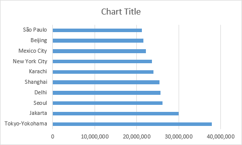
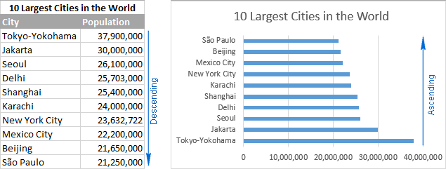
Let’s illustrate this with a simple data set. The worksheet contains a list of the 10 largest cities in the world, arranged in descending order of population. In a bar chart, the data will be arranged from top to bottom in ascending order.
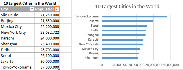
Чтобы на диаграмме Excel данные расположились от больших к меньшим сверху вниз, достаточно упорядочить их в исходной таблице в обратном порядке, т.е. от меньших к большим:
If for some reason sorting the data in the table is not possible, then the following will show a way to change the order of the data in the Excel chart without changing the order of the data in the original table.
We arrange the data in the Excel bar chart in ascending/descending order without sorting the source data
If the order of the source data on the worksheet matters and cannot be changed, let’s make the chart bars appear in exactly the same order. It’s simple – you just need to enable a couple of additional options in the settings settings.
- In an Excel bar chart, right-click on any of the vertical axis labels and from the context menu, click Axis Format (Format Axis). Or just double click on the vertical axis labels.
- In the panel that appears, in the section Axis parameters (Axis Options) configure the following options:
- In a group Пересечение с горизонтальной осью (Horizontal axis crosses) select At the point with the highest category value (At maximum category).
- In a group Axis position (Axis position) select Reverse order of categories (Categories in reverse order).
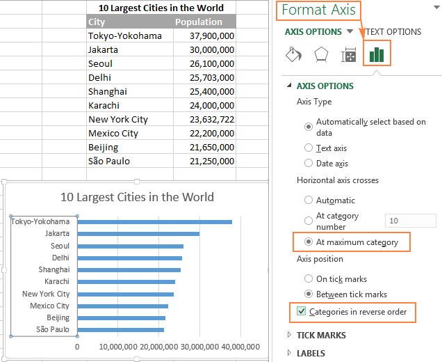
Готово! Данные в линейчатой диаграмме Excel немедленно выстроятся в том же порядке, что и в исходной таблице, – по возрастанию или по убыванию. Если порядок исходных данных будет изменён, то данные на диаграмме автоматически повторят эти изменения.
Change the order of data series in a bar chart
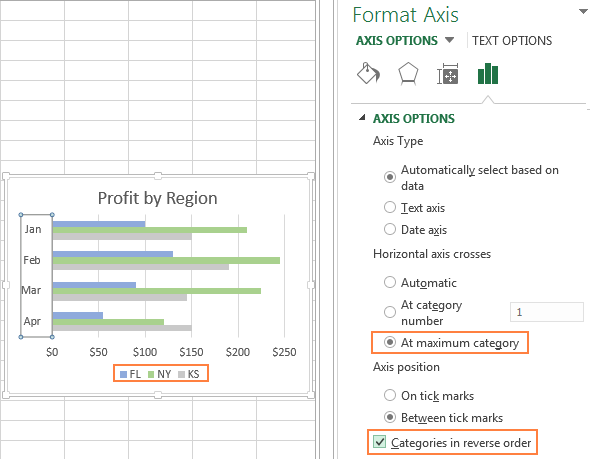
If an Excel bar chart contains multiple data series, they are also built in reverse order by default. Pay attention to the figure below: the regions in the table and in the diagram are in opposite order.
To arrange data series in a bar chart in the same order as in a worksheet, use the options At the point with the highest category value (At maximum category) и Reverse order of categories (Categories in reverse order), как мы сделали это в предыдущем примере. Порядок построения категорий при этом также изменится, как видно на следующем рисунке:
Если нужно расставить ряды данных в линейчатой диаграмме в порядке, отличающемся от порядка данных на рабочем листе, то это можно сделать при помощи:
Changing the Order of Data Series Using the Select Data Source Dialog Box
This method allows you to change the order of plotting data series in a bar chart for each series separately and at the same time keep the order of the source data on the worksheet unchanged.
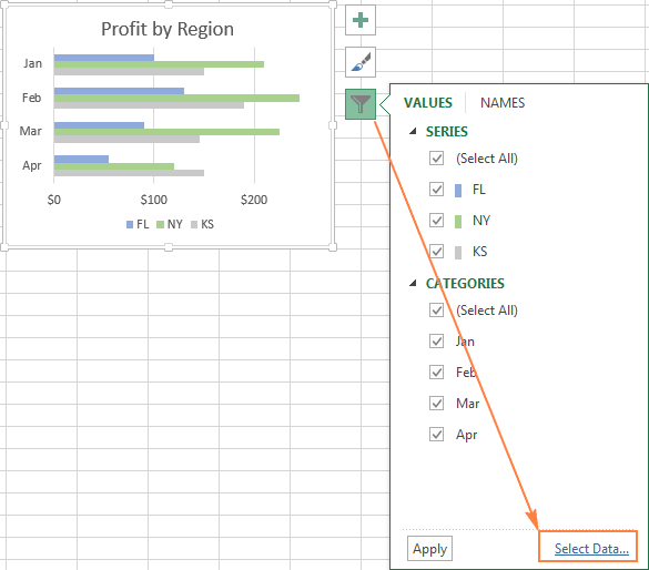
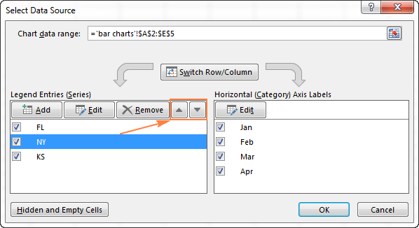
- Select a chart to display a group of tabs on the Menu Ribbon Working with charts (ChartTools). Open a tab Constructor (Design) and in the section Data (Data) click the button Select data (Select Data). Or click the icon Chart Filters (Chart Filters) to the right of the chart and click the link Select data (Select Data) at the bottom of the menu that opens.
- In the dialog box Selecting a data source (Select Data Source) select the data series for which you want to change the construction order, and move it up or down using the arrows:
Изменяем порядок рядов данных при помощи формул
Each data series in Excel charts (not just bar charts – any chart) is defined by a formula, so you can change the data series by changing its formula. Within the framework of this article, we are only interested in the last argument of this formula, which determines the order in which the series are constructed. You can read more about the data series formula in this article.
For example, the gray bar chart data series in the following example is in third place.
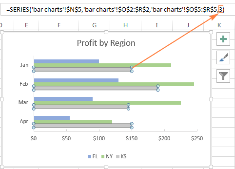
Чтобы изменить порядок построения данного ряда данных, выделите его в диаграмме, затем в строке формул измените последний аргумент формулы на любое другое число. В нашем примере, чтобы переместить ряд данных на одну позицию вверх, введите «2», а чтобы сделать его первым в диаграмме, введите «1» в качестве последнего аргумента.
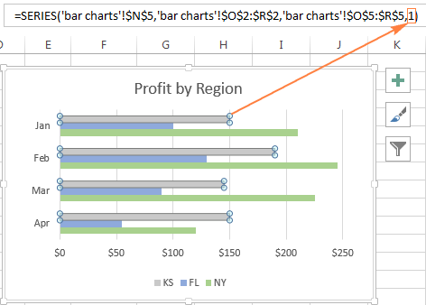
Как и настройка параметров в диалоговом окне Selecting a data source (Select Data Source), editing the data series formula changes the order of the data series only in the chart; the original data on the worksheet remains unchanged.
This is how a bar chart is built in Excel. For those who want to learn more about Excel charts, I recommend that you study the articles from this section of the site. Thank you for your attention!