


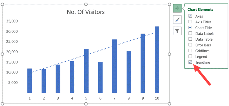
This example will teach you how to add a trend line to an Excel chart.
- Right click on the data series and in the context menu click Add trend line (Add Trendline).
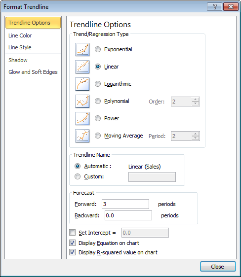
- Click the tab Trendline Options (Trend/Regression Type) and select Linear (Linear).
- Specify the number of periods to include in the forecast – enter the number “3” in the field Forward to (Forward).
- Tick the options Show equation on chart (Display Equation on chart) и Put on the diagram the value of the approximation confidence (Display R-squared value on chart).

- Press Close (Close).
Result:
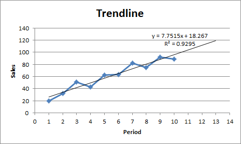
Explanation:
- Excel uses the least squares method to find the line that best fits the elevations.
- The R-squared value is 0,9295 which is a very good value. The closer it is to 1, the better the line fits the data.
- The trend line gives an idea of the direction in which the sales are going. During the period 13 sales may reach 120 (this is a forecast). This can be verified using the following equation:
y = 7,7515*13 + 18,267 = 119,0365