How to Add a Legend to an Excel 2010 Chart

In Microsoft Office Excel, you can quickly build a chart on a compiled table array to reflect its main characteristics. It is customary to add a legend to the diagram in order to characterize the information depicted on it, to give them names. This article will discuss the methods of adding a legend to a chart in Excel 2010.

How to build a chart in Excel from a table

First you need to understand how the diagram is built in the program in question. The process of its construction is conditionally divided into the following stages:

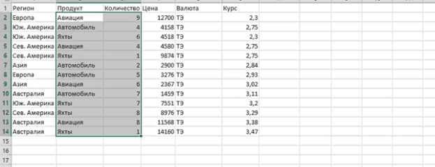
1. In the source table, select the desired range of cells, columns for which you want to display the dependency.

2. Go to the “Insert” tab in the upper column of the tools of the main menu of the program.
3. In the “Diagrams” block, click on one of the options for the graphical representation of the array. For example, you can choose a pie chart or a bar chart.

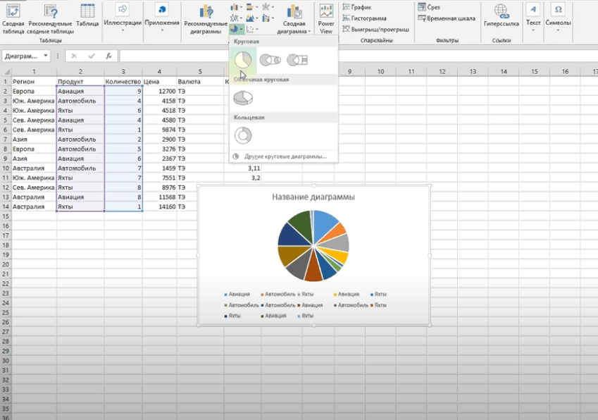
4. After completing the previous step, a window with the constructed chart should appear next to the original plate on the Excel worksheet. It will reflect the relationship between the values ​​selected in the array. So the user will be able to visually assess the differences in values, analyze the graph and draw a conclusion from it.

Pay attention! Initially, an “empty” chart will be built without a legend, data label, and legend. This information can be added to the chart if desired.

How to add a legend to a chart in Excel 2010 in the standard way

This is the simplest method for adding a legend and will not take the user much time to implement. The essence of the method is to do the following steps:

1. Build a diagram according to the above scheme.
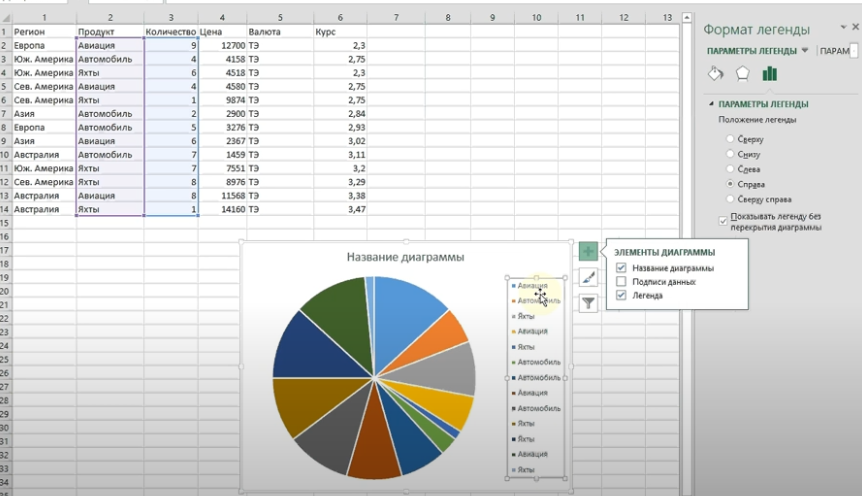
2. With the left mouse button, click on the green cross icon in the toolbar to the right of the chart.
3. In the window of available options that opens, next to the “Legend” line, check the box to activate the function.

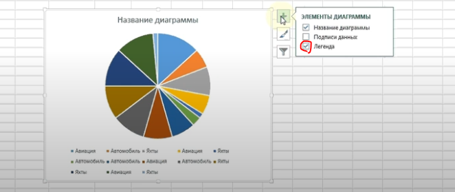
4. Analyze chart. Labels of elements from the original table array should be added to it.
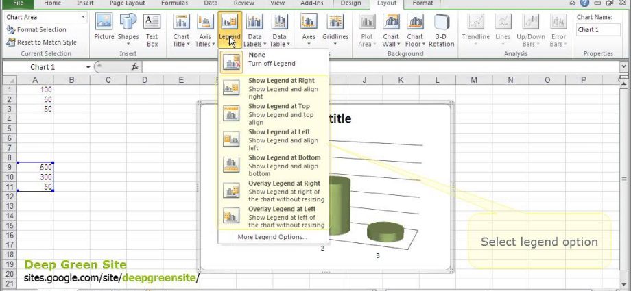
5. If necessary, you can change the location of the graph. To do this, left-click on the legend and select another option for its location. For example, Left, Bottom, Top, Right, or Top Left.

How to change legend text on a chart in Excel 2010

The legend captions can be changed if desired by setting the appropriate font and size. You can do this by following the instructions below:

1. Build a chart and add a legend to it according to the algorithm discussed above.
2. Change the size, font of the text in the original table array, in the cells on which the graph itself is built. When formatting text in table columns, the text in the chart legend will automatically change.
3. Check result.

Important! In Microsoft Office Excel 2010, it is problematic to format the legend text on the chart itself. It is easier to use the considered method by changing the data of the table array on which the graph is built.

How to complete the chart

In addition to the legend, there are some more data that can be reflected in the plot. For example, her name. To name the constructed object, you must proceed as follows:

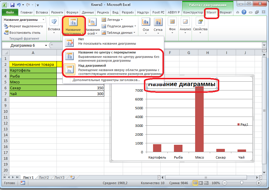
1. Build a diagram according to the original plate and move to the “Layout” tab at the top of the main menu of the program.
2. The Chart Tools pane opens, with several options available for editing. In this situation, the user needs to click on the “Chart Name” button.
3. In the drop-down list of options, select the type of title placement. It can be placed in the center with an overlap, or above the chart.

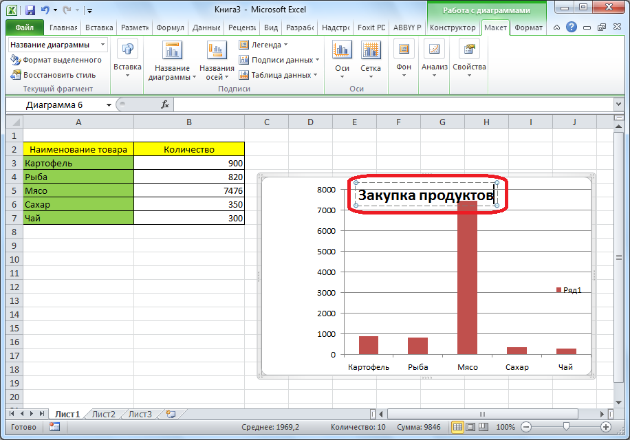
4. After performing the previous manipulations, the plotted chart will display the inscription “Chart Name”. The user will be able to change it by manually typing any other combination of words from the computer keyboard that matches the meaning of the original table array.

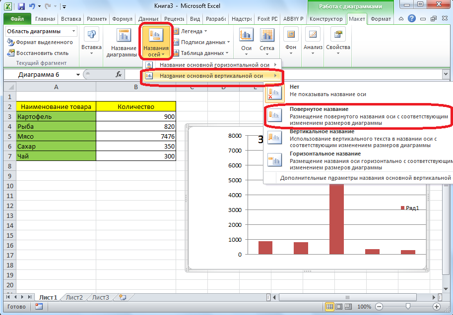
5. It is also important to label the axes on the chart. They are signed in the same way. In the block for working with charts, the user will need to click on the “Axis Names” button. In the drop-down list, select one of the axes: either vertical or horizontal. Next, make the appropriate change for the selected option.

Additional Information! According to the scheme discussed above, you can edit the chart in any version of MS Excel. However, depending on the year the software was released, the steps for setting up charts may vary slightly.

Alternative Method to Change Chart Legend in Excel

You can edit the text of labels on the chart using the tools built into the program. To do this, you need to follow a few simple steps according to the algorithm:

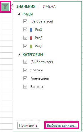
1. With the right mouse button, click on the required word of the legend in the constructed diagram.
2. In the context type window, click on the “Filters” line. This will open the Custom Filters window.
3. Click the Select Data button at the bottom of the window.

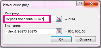
4. In the new “Select Data Sources” menu, you must click on the “Edit” button in the “Legend Elements” block.
5. In the next window, in the “Row Name” field, enter a different name for the previously selected element and click on “OK”.

6. Check result.

Conclusion

Thus, the construction of a legend in Microsoft Office Excel 2010 is divided into several stages, each of which needs to be studied in detail. Also, if desired, the information on the chart can be quickly edited. The basic rules for working with charts in Excel have been described above.