


Contents
If you are at least familiar with the function VPR (VLOOKUP) (if not, then first run here), then you should understand that this and other functions similar to it (VIEW, INDEX and SEARCH, SELECT, etc.) always give as a result value – the number, text or date that we are looking for in the given table.
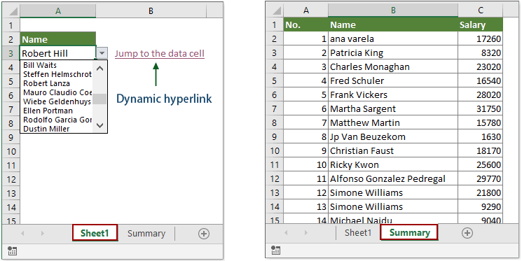
But what if, instead of a value, we want to get a live hyperlink, by clicking on which we could instantly jump to the found match in another table to look at it in a general context?
Let’s say we have a large order table for our customers as input. For convenience (although this is not necessary), I converted the table to a dynamic “smart” keyboard shortcut Ctrl+T and gave on the tab Constructor (Design) her name tabOrders:
On a separate sheet Consolidated I built a pivot table (although it doesn’t have to be exactly a pivot table – any table is suitable in principle), where, according to the initial data, the sales dynamics by months for each client is calculated:
Let’s add a column to the order table with a formula that looks up the name of the customer for the current order on the sheet Consolidated. For this we use the classical bunch of functions INDEX (INDEX) и MORE EXPOSED (MATCH):
Now let’s wrap our formula into a function CELL (CELL), which we will ask to display the address of the found cell:
And finally, we put everything that has turned out into a function HYPERLINK (HYPERLINK), which in Microsoft Excel can create a live hyperlink to a given path (address). The only thing that is not obvious is that you will have to glue the hash sign (#) at the beginning to the received address so that the link is correctly perceived by Excel as internal (from sheet to sheet):
Now, when you click on any of the links, we will instantly jump to the cell with the name of the company on the sheet with the pivot table.
To make it really good, let’s slightly improve our formula so that the transition occurs not to the client’s name, but to a specific numerical value exactly in the month column when the corresponding order was completed. To do this, we must remember that the function INDEX (INDEX) in Excel is very versatile and can be used, among other things, in the format:
=INDEX( XNUMXD_range; Line_number; Column_number )
That is, as the first argument, we can specify not the column with the names of companies in the pivot, but the entire data area of the pivot table, and as the third argument, add the number of the column we need. It can be easily calculated by the function MONTH (MONTH), which returns the month number for the deal date:
Improvement 2. Beautiful link symbol
Second function argument HYPERLINK – the text that is displayed in a cell with a link – can be made prettier if you use non-standard characters from Windings, Webdings fonts and the like instead of the banal signs “>>”. For this you can use the function SYMBOL (CHAR), which can display characters by their code.
So, for example, character code 56 in the Webdings font will give us a nice double arrow for a hyperlink:
Improvement 3. Highlight current row and active cell
Well, for the final victory of beauty over common sense, you can also attach to our file a simplified version of highlighting the current line and the cell that we follow the link to. This will require a simple macro, which we will hang to handle the selection change event on the sheet Consolidated.
To do this, right-click on the sheet tab Summary and select the command View code (View code). Paste the following code into the Visual Basic editor window that opens:
Private Sub Worksheet_SelectionChange(ByVal Target As Range) Cells.Interior.ColorIndex = -4142 Cells(ActiveCell.Row, 1).Resize(1, 14).Interior.ColorIndex = 6 ActiveCell.Interior.ColorIndex = 44 End Sub
As you can easily see, here we first remove the fill from the entire sheet, and then fill the entire line in the summary with yellow (color code 6), and then orange (code 44) with the current cell.
Now, when any cell inside the summary cell is selected (it doesn’t matter – manually or as a result of clicking on our hyperlink), the entire row and cell with the month we need will be highlighted:
Beauty 🙂
PS Just remember to save the file in a macro-enabled format (xlsm or xlsb).
- Creating external and internal links with the HYPERLINK function
- Creating emails with the HYPERLINK function