


Contents
In this little lesson you will find a lot of useful information about percentage format in Excel. You will learn how to change the format of existing data to Percentage, how to set the display of percentages in a cell, as well as how to automatically change numbers to percentages when manually entered.
In Microsoft Excel, displaying values as percentages is very easy. To do this, select one or more cells and click the button Percent Style (percentage format) in the section Number (Number) tabs Home (Home):
You can do it even faster by pressing the keyboard shortcut Ctrl+Shift+%. Excel will remind you of this combination each time you hover over the button. Percent Style (percentage format).
Yes, Percent Format in Excel can be set in one click. But the result will be significantly different depending on whether you are applying formatting to existing values or empty cells.
Format existing values as percentages
When you apply Percent Format For cells that already contain numeric values, Excel multiplies those values by 100 and adds a percent sign (%) at the end. From the point of view of Excel, this is correct, since 1% is essentially one hundredth.
However, sometimes this leads to unexpected results. For example, if cell A1 contains the number 20 and you apply to this cell Percent Format, then as a result you will get 2000%, and not 20% as you probably wanted.
How to prevent the error:
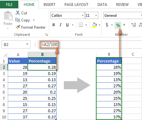
- If a cell in your table contains numbers in the usual number format, and you need to turn them into Percentage, first divide these numbers by 100. For example, if your initial data is written in column A, you can enter the formula in cell B2 =A2/100 and copy it to all the necessary cells of column B. Next, select the entire column B and apply to it Percent Format. The result should be something like this:
 You can then replace the formulas in column B with values, then copy them to column A and delete column B if you no longer need it.
 - If you only need to convert some of the values to percentage format, you can enter them manually by dividing the number by 100 and writing it as a decimal. For example, to get the value 28% in cell A2 (see the figure above), enter the number 0.28, and then apply to it Percent Format.
 You can then replace the formulas in column B with values, then copy them to column A and delete column B if you no longer need it.
Apply percentage format to empty cells
We saw how the display of already existing data in a Microsoft Excel spreadsheet changes when you change the simple number format to Percentage. But what happens if you first apply to a cell Percent Format, and then enter a number into it manually? This is where Excel can behave differently.
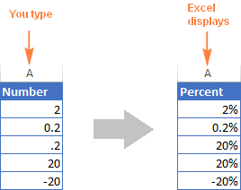
- Any number equal to or greater than 1 will simply be written with a % sign. For example, the number 2 would be written as 2%; 20 – like 20%; 2,1 – like 2,1% and so on.
- Numbers less than 1 written without a 0 to the left of the decimal point will be multiplied by 100. For example, if you type ,2 into a cell with percentage formatting, you will see a value of 20% as a result. However, if you type on the keyboard 0,2 in the same cell, the value will be written as 0,2%.
Display numbers as percentages immediately as you type
If you enter the number 20% (with a percent sign) into a cell, Excel will understand that you want to write the value as a percentage and automatically change the format of the cell.
Important notice!
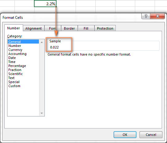
When using percentage formatting in Excel, please remember that this is nothing more than a visual representation of the actual mathematical value stored in a cell. In fact, the percentage value is always stored as a decimal.
In other words, 20% is stored as 0,2; 2% is stored as 0,02 and so on. When various calculations are made, Excel uses these values, i.e. decimal fractions. Keep this in mind when formulating formulas that refer to cells with percentages.
To see the real value contained in a cell that has Percent Format:
- Right-click on it and from the context menu select Format Cells or press combination Ctrl + 1.
- In the dialog box that appears Format Cells (Cell Format) take a look at the area sample (Sample) tab Number (Number) in category General (General).
Tricks when displaying percentages in Excel
It seems that calculating and displaying data as a percentage is one of the simplest tasks we do with Excel. But experienced users know that this task is not always so simple.
1. Set the display to the desired number of decimal places
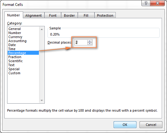
When Percent Format applied to numbers, Excel 2010 and 2013 displays their value rounded to a whole number, and in some cases this can be misleading. For example, set a percentage format to an empty cell and enter a value of 0,2% in the cell. What happened? I see 0% in my table, although I know for sure that it should be 0,2%.
To see the real value and not the round value, you need to increase the number of decimal places that Excel should show. For this:
- Open a dialog box Format Cells (Format cells) using the context menu, or press the key combination Ctrl + 1.
- Select a category Percentage (Percentage) and set the number of decimal places displayed in the cell as you wish.
- When everything is ready, click OKfor the changes to take effect.
2. Highlight Negative Values with Formatting
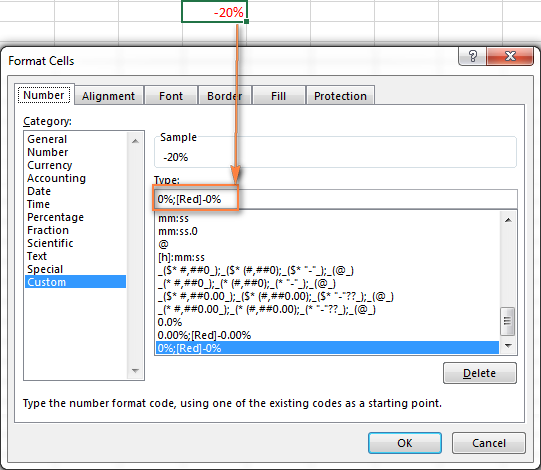
If you want negative values to be displayed differently, such as in red font, you can set a custom number format. Reopen the dialog Format Cells (Format cells) and go to the tab Number (Number). Select a category Custom (All Formats) and enter in the field type one of the following lines:
- 00%;[Red]-0.00% or 00%;[Red]-0,00% — display negative percentage values in red and show 2 decimal places.
- 0%;[Red]-0% or 0%; [Krasleepy]-0% — display negative percentage values in red and do not show values after the decimal point.
You can learn more about this formatting method in the Microsoft reference, in the topic on displaying numbers in percentage format.
3. Format Negative Percentage Values in Excel with Conditional Formatting
Compared to the previous method, conditional formatting in Excel is a more flexible method that allows you to set any format for a cell containing a negative percentage value.
The easiest way to create a conditional formatting rule is to go to the menu Conditional formatting > Highlight cells rules > Less than (Conditional Formatting > Cell Selection Rules > Less Than…) and enter 0 in the field Format cells that are LESS THAN (Format cells that are LESS)
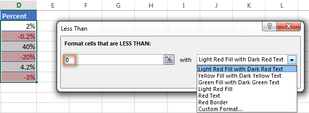
Next, in the drop-down list, you can select one of the proposed standard options or click Custom Format (Custom Format) at the end of this list and customize all cell format details as you like.
Here are some options for working with Percentage format data opens Excel. I hope that the knowledge gained from this lesson will save you from unnecessary headaches in the future. In the following articles, we will dive deeper into the topic of percentages in Excel. You’ll learn which methods you can use to calculate interest in Excel, learn formulas for calculating percent change, percent of total, compound interest, and more.
Stay tuned and happy reading!