


Contents
- 3 Ways to Customize Chart Options in Excel
- How to add a title to an Excel chart
- Setting up chart axes in Excel
- Adding Data Labels to an Excel Chart
- Adding, Removing, Moving, and Customizing the Format of a Chart Legend
- Show and hide the grid in an Excel chart
- Hiding and editing data series in an Excel chart
- Change the chart type and style
- Changing chart colors
- How to swap the x and y axes of a chart
- How to rotate a chart in Excel from left to right
What is the first thing we think about after creating a chart in Excel? About how to give the diagram exactly the look we imagined when we got down to business!
In modern versions of Excel 2013 and 2016, customizing charts is easy and convenient. Microsoft has gone to great lengths to make the setup process simple and the required options easily accessible. Later in this article, we’ll show you some easy ways to add and customize all the basic chart elements in Excel.
3 Ways to Customize Chart Options in Excel
If you had a chance to read our previous article on how to create a chart in Excel, then you already know that you can access the basic charting tools in one of three ways:
- Select chart and use tabs from group Working with charts (Chart Tools) – Constructor (Design) Framework (Format).
- Right-click on the chart element you want to customize and select the desired command from the context menu.
- Use special icons that appear near the upper right corner of the chart when you click on it with the mouse.
Even more options are in the panel Chart Area Format (Format Chart), which appears on the right side of the worksheet when you click More options (More options) in the context menu of the diagram or on the tabs of the group Working with charts (Chart Tools).
Tip: To immediately open the desired section of the panel for setting the chart parameters, double-click on the corresponding element on the chart.
Armed with this basic knowledge, let’s take a look at how we can modify the various elements of a chart in Excel to give it exactly the look we want it to look like.
How to add a title to an Excel chart
In this section, we’ll show you how to add a title to a chart in different versions of Excel and show you where the main charting tools are. In the rest of the article, we will consider examples of work only in the newest versions of Excel 2013 and 2016.
Adding a Title to a Chart in Excel 2013 and Excel 2016
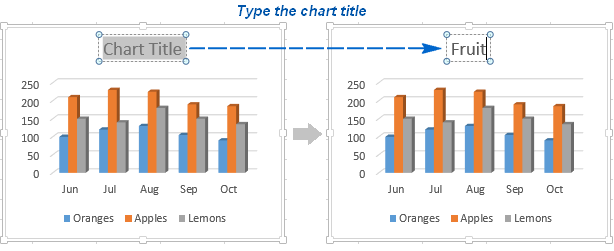
In Excel 2013 and Excel 2016, when you create a chart, the text “Chart title“. To change this text, simply select it and enter your own name:
You can also link the chart title to a cell on the sheet using a link so that the title is automatically updated whenever the contents of the linked cell change. How to do this is described below.
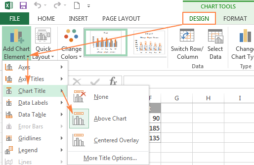
If for some reason the title was not added automatically, then click anywhere in the diagram to bring up a group of tabs Working with charts (ChartTools). Open a tab Constructor (Design) and press Add Chart Element (Add Chart Element) > Chart title (Chart Title) > Above chart (Above Chart) or Center (overlay) (Centered Overlay).
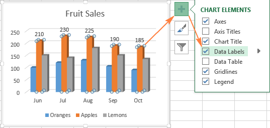
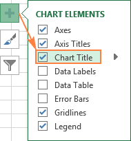
Or click the icon Chart elements (Chart Elements) near the upper right corner of the chart and check the box Chart title (Chart Title).
next to the option Chart title (Chart Title), you can click the arrow pointing to the right (see the figure above) and select one of the options:
- Above chart (Above Chart) – the name is placed above the chart construction area, while the chart size is reduced; this option is used by default.
- Center (overlay) (Centered Overlay) – the centered title is superimposed on top of the plotting area, while the chart size does not change.
For more options, click the tab Constructor (Design) and press Add Chart Element (Add Chart Element) > Chart title (Chart Title) > Additional header options (More options). Or click the icon Chart elements (Chart Elements), then Chart title (Chart Title) > More options (More Options).
Button press More options (More Options), in both cases, opens the panel Chart Title Format (Format Chart Title) on the right side of the worksheet, where you can find the options you want.
Adding a Title to a Chart in Excel 2010 and Excel 2007
To add a title to a chart in Excel 2010 and earlier, follow these steps:
- Click anywhere in the Excel chart to bring up a group of tabs on the Menu Ribbon Working with charts (Chart Tools).
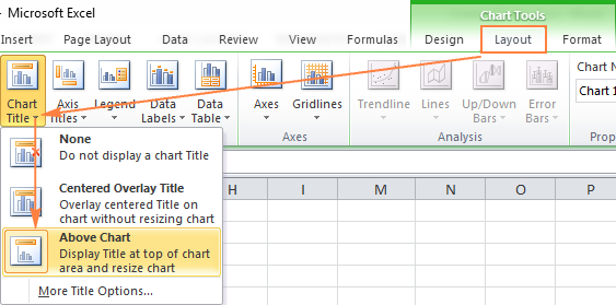
- On the Advanced tab Layout (Layout) click Chart title (Chart Title) > Above chart (Above Chart) or Center (overlay) (Centered Overlay).

Associating a chart title with a worksheet cell
Charts of various types in Excel are most often created with alt text instead of a title. To set your own name for the chart, you can either select the chart field and enter the text manually, or link it to any cell in the worksheet containing, for example, the name of the table. In this case, the title of the Excel chart will be automatically updated every time the contents of the linked cell change.
To link a chart title to a worksheet cell:
- Highlight the title of the chart.
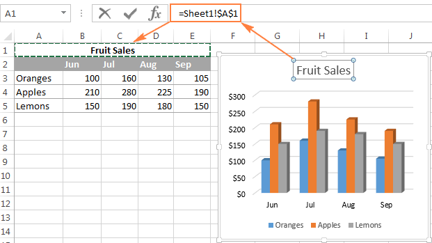
- In the formula bar, type an equal sign (=), click on the cell containing the desired text, and press Enter.
In this example, we are linking the title of an Excel chart to a cell A1. You can select two or more cells (for example, multiple column headers) and the resulting chart title will show the contents of all the selected cells.
Moving the title in the chart
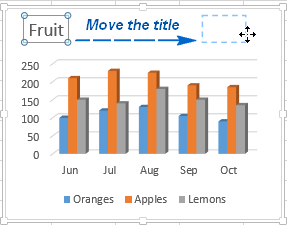
If you want to move the chart title to another location, select it and drag it with your mouse:
Removing the chart title
If the Excel chart does not need a title, then it can be removed in two ways:
- On the Advanced tab Constructor (Design) click Add Chart Elements (Add Chart Element) > Chart title (Chart Title) > No (None).
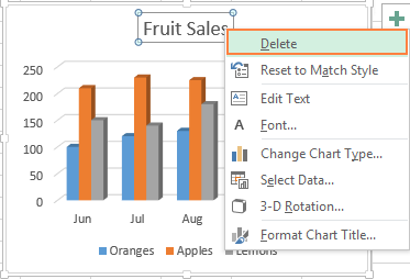
- Right-click on the chart name and in the context menu click Remove (Delete).
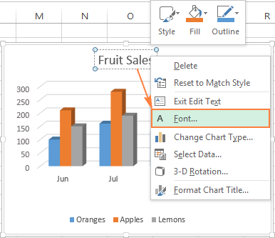
Change the font and design of the chart title
To change the font of the chart title in Excel, right-click on it and click Font (Font) in the context menu. A dialog box of the same name will open, in which you can configure various font settings.
If you need more detailed settings, select the name of the diagram, open the tab Framework (Format) and play around with the various options. Here is how, for example, you can transform the chart title using the Menu Ribbon:
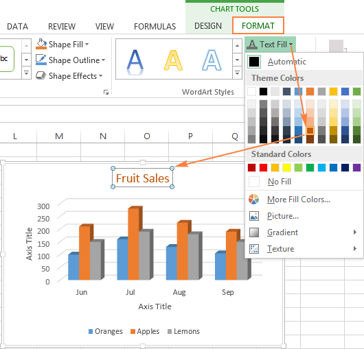
In the same way, you can change the appearance of other chart elements, such as axis titles, axis labels, and the chart legend.
For more information about this, see the article How to add a title to a chart in Excel.
Setting up chart axes in Excel
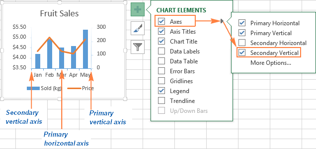
For most chart types in Excel vertical axis (it is also the value axis or the Y axis) and horizontal axis (it is also the category axis or the X axis) are added automatically when creating a chart.
To hide or show the chart axes, click on the icon Chart elements (Chart Elements), then click the arrow in the row Axes (Axes) and tick the axes you want to show, or uncheck the boxes next to those you want to hide.
For some chart types, such as combo charts, a secondary axis may be shown.
When creating XNUMXD charts, you can display depth axis:
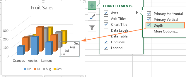
For each element of the chart axes in Excel, you can configure various parameters (we’ll talk about this in more detail later):
Adding Axis Titles to a Chart
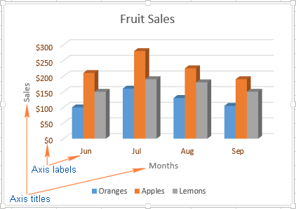
When creating a chart in Excel, you can add titles for the vertical and horizontal axes to make it easier for users to understand what data is shown in the chart. To add axis titles, you need to do the following:
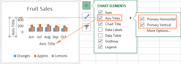
- Click anywhere in the Excel chart, then click the icon Chart elements (Chart Elements) and check the box Axis names (Axis Titles). If you only want to show the title for one of the axes (either vertical or horizontal), click the arrow on the right and uncheck one of the boxes.
- Click on the chart in the axis title text field and enter the text.
To customize the appearance of the axis title, right-click on it and in the context menu click Axis name format (Format Axis Title). This will open a panel of the same name with a large selection of custom design options. You can also use the options offered on the tab Framework (Format) Menu ribbons, as we did when setting the chart title options.
Associating axis titles with given worksheet cells
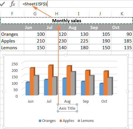
Like the chart title, the axis title can be linked to a given worksheet cell using a link so that the title is updated automatically when the data in the linked cell changes.
To create such a link, select the axis name and in the formula bar enter the equal sign (=), then click on the cell to which you want to link the axis name, and click Enter.
Change the scale of the chart axis
Microsoft Excel automatically determines the minimum and maximum values, as well as the units for the vertical axis, based on what data is used to build the chart. If necessary, you can set your own more suitable parameters for the vertical axis.
- Select the vertical axis of the chart and click on the icon Chart elements (Chart Elements).
- Click the arrow in the row Axes (Axis) and in the menu that appears, select More options (More options). The panel will open Axis Format (Format Axis).
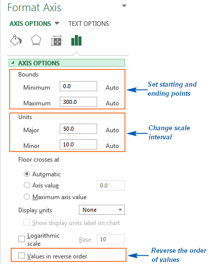
- In section Axis parameters (Axis Options) do one of the following:
- To set the start and end values of the vertical axis, enter the appropriate values in the fields Minimum (Minimum) or Maximum (Maximum).
- To change the axis scale, enter values in the fields Major divisions (Major) и Intermediate divisions (Minor).
- To reverse axis values, check the box Reverse order of values (Values in reverse order).
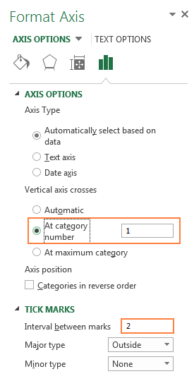
The horizontal axis, unlike the vertical one, often has text data labels rather than numeric ones, so this axis has fewer scale settings. However, you can change the number of categories to be shown between the labels, the order of the categories, and the point where the two axes intersect:
Changing the number format for axis labels
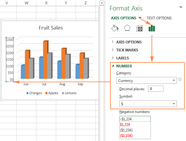
If you want the numbers in the axis labels to be displayed as currencies, percentages, times, or in some other format, right-click on the labels and in the context menu click Axis Format (Format Axis). In the panel that opens, go to the section Number (Number) and select one of the available number formats:
Tip: To set the format of the source data for numbers (the one in the cells of the worksheet), check the box Link to source (Linked to source). If you can’t find the section Number (Number) in panels Axis Format (Format Axis), check that the value axis is selected on the chart (this is usually the vertical axis).
Adding Data Labels to an Excel Chart
To make the chart easier to understand in Excel, add data labels that show detailed information about the data series. Depending on what you want users to pay attention to, you can add labels to a single data series, to all series, or to individual points.
- Click on the data series for which you want to add labels. To add a label to only one data point, click again on that data point.
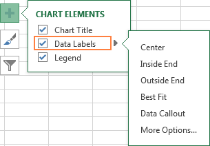
- Click on the icon Chart elements (Chart Elements) and check the box Data Signatures (Data Labels).
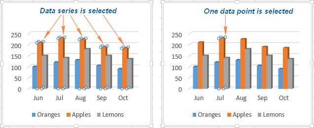
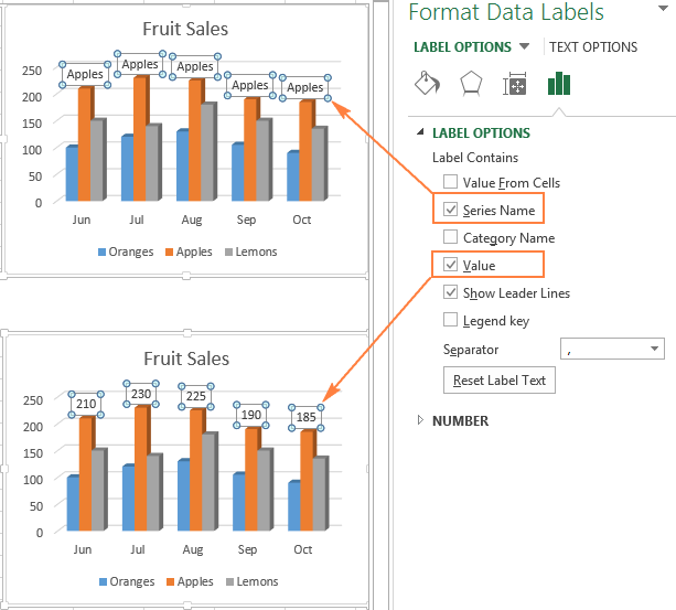
For example, this is how our Excel chart looks like with labels for one of the data series.

In some cases, you can choose how labels will be placed. To do this, click the arrow in the line Data Signatures (Data Labels) and select the appropriate option. To show labels inside floating text fields, select Callout Data (Data Callout).
How to change the data displayed in labels
To change the content of the data labels on the chart, click on the icon Chart elements (Chart Elements) > Data Signatures (Data Labels) > More options (More options). The panel will open Data Label Format (Format Data Labels) on the right side of the worksheet. On the tab Signature Options (Label Options) in the section Include in Signature (Label Contains) choose from the options provided.
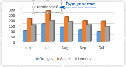
If you want to add custom text to one of the data points, click on that point’s label, then click again to keep only that label selected, and again on the label’s text to select it. Next, enter your own text.
If it turns out that too many labels overload the Excel chart, then you can delete any of them. Click on the signature with the right mouse button and in the context menu click Remove (Delete).
Tips for working with data labels:
- To change the position of one signature, simply drag it with the mouse to the desired location.
- To change the font color and fill of data labels, select them, then click the tab Framework (Format) and configure the formatting options you want.
Adding, Removing, Moving, and Customizing the Format of a Chart Legend
When you create a chart in Excel 2013 and Excel 2016, a legend is added at the bottom of the chart area by default. In Excel 2010 and earlier, to the right of the construction area.
To remove the legend, click the icon Chart elements (Chart Elements) near the upper right corner of the chart and uncheck the box Legend (Legend).
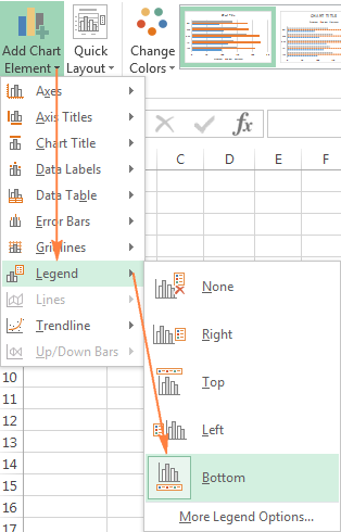
To move the chart legend to a different location, select the chart, open the tab Constructor (Design), click Add Chart Element (Add Chart Element) > Legend (Legend) and select a new position for the legend. To remove the legend, click No (None).
Another way to move the legend is to double-click on it and select the desired position in the section. Legend options (Legend Options) panels Legend Format (Format Legend).
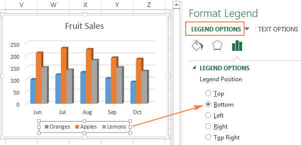
To customize the formatting of the legend, there are many options on the tabs Shading and Borders (Fill & Line) and Effects (Effects) panels Legend Format (Format Legend).
Show and hide the grid in an Excel chart
In Excel 2013 and 2016, showing or hiding the grid is a matter of seconds. Just click on the icon Chart elements (Chart Elements) and check or uncheck the box Сетка (Gridlines).
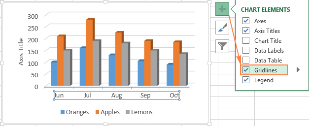
Microsoft Excel automatically determines which gridlines are best for a given chart type. For example, a bar chart will show major vertical lines, while a column chart will show major horizontal grid lines.
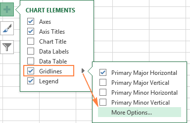
To customize the type of grid lines displayed, click the right arrow in the row Сетка (Gridlines) and select the appropriate one from the proposed options, or click More options (More Options) to open the panel Main Grid Line Format (Major Gridlines).
Hiding and editing data series in an Excel chart
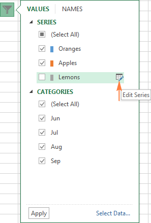
When an Excel chart shows a lot of data, sometimes it is necessary to temporarily hide part of the series in order to focus on the ones you need at the moment.
To do this, click the icon to the right of the graph. Chart Filters (Chart Filters) and uncheck those rows and/or categories that you want to hide.
To edit a data series, press the button Change row (Edit Series) to the right of its name. The button appears when you move the mouse over the name of this row. This will highlight the corresponding row on the graph, so you can easily see which element will be edited.
Change the chart type and style
If the chart you created is not the best fit for the data you are displaying, you can easily change the chart type. To do this, select the diagram, open the tab Insert (Insert) and in section Diagrams (Charts) select a different chart type.
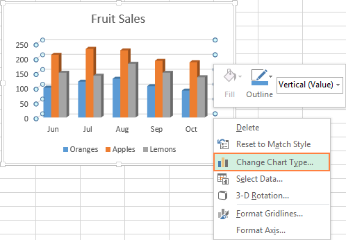
Another way is to right-click anywhere in the chart and from the context menu click Change chart type (Change Chart Type).
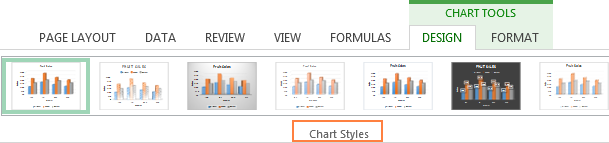
In order to quickly change the style of the created chart, click the icon Chart styles (Chart Styles) to the right of the construction area and select the appropriate one from the proposed styles.
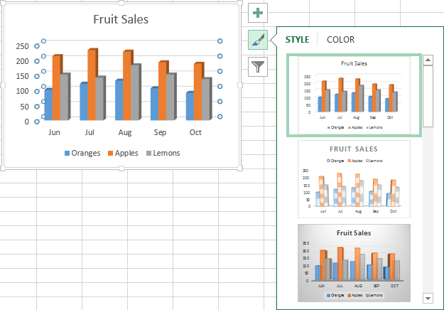
Or choose one of the styles in the section Chart styles (Charts Styles) tab Constructor (Design):
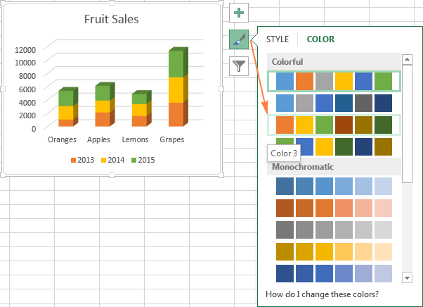
Changing chart colors
To change the color theme of a chart in Excel, click the icon Chart styles (Chart Styles), open the tab Color (Color) and select one of the suggested color themes. The chosen colors will immediately be applied to the diagram, and you can immediately evaluate whether it looks good in the new color.
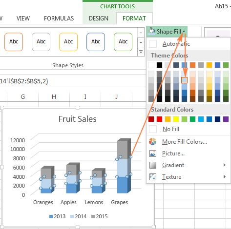
To select a color for each series individually, select the data series in the chart, open the tab Framework (Format) and in the section Shape styles (Shape Styles) click Shape fill (Shape Fill).
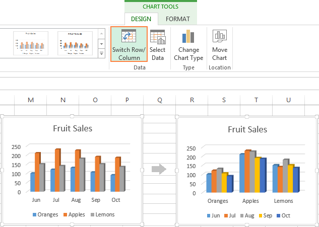
How to swap the x and y axes of a chart
When creating a chart in Excel, the orientation of the data series is determined automatically based on the number of rows and columns of the source data on which the chart is built. In other words, Microsoft Excel independently decides how best to draw a graph for the selected rows and columns.
If the default arrangement of rows and columns on the chart does not suit you, then you can easily swap the horizontal and vertical axes. To do this, select the diagram and on the tab Constructor (Design) click Row column (Switch Row/Column).
How to rotate a chart in Excel from left to right
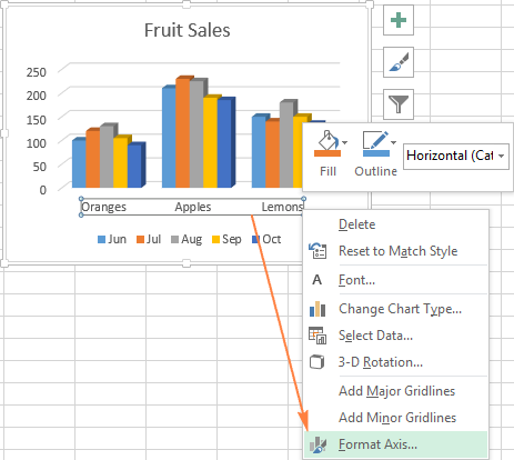
Have you ever created a chart in Excel and only at the very end realized that the data points are in the opposite order of what you wanted to get? To fix this situation, you need to reverse the order in which the categories are built in the diagram, as shown below.
Right click on the horizontal axis of the chart and click Axis Format (Format Axis) in the context menu.
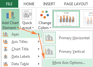
If you are more accustomed to working with the Ribbon, open the tab Constructor (Design) and press Add Chart Element (Add Chart Element) > Axes (Axes) > Additional Axis Options (More Axis Options).
Either way, a panel will appear. Axis Format (Format Axis) where on the tab Axis parameters (Axis Options) you need to tick the option Reverse order of categories (Categories in reverse order).
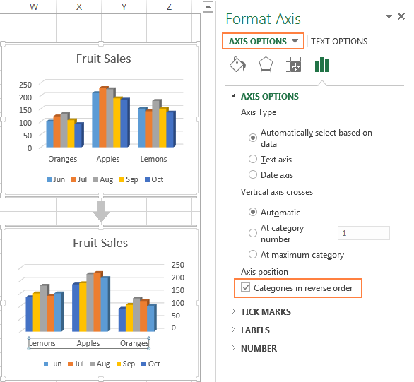
In addition to flipping a chart in Excel from left to right, you can change the order of categories, values, or data series in a chart, reverse the plotting order of data points, rotate a pie chart to any angle, and more. A separate article is devoted to the topic of rotating charts in Excel.
Today you learned about how you can customize charts in Excel. Of course, this article only allows you to scratch the surface of the topic of settings and formatting charts in Excel, although much more can be said about this. In the next article, we will build a chart from data that is on various worksheets. In the meantime, I recommend that you practice to consolidate the knowledge gained today.