


Contents
When mentioning databases (DB), the first thing that comes to mind, of course, is all sorts of buzzwords like SQL, Oracle, 1C, or at least Access. Of course, these are very powerful (and expensive for the most part) programs that can automate the work of a large and complex company with a lot of data. The trouble is that sometimes such power is simply not needed. Your business may be small and with relatively simple business processes, but you also want to automate it. And it is for small companies that this is often a matter of survival.
To begin with, let’s formulate the TOR. In most cases, a database for accounting, for example, classic sales should be able to:
- keep in the tables information on goods (price), completed transactions and customers and link these tables to each other
- have comfortable input forms data (with drop-down lists, etc.)
- automatically fill in some data printed forms (payments, bills, etc.)
- issue the necessary reports to control the entire business process from the point of view of the manager
Microsoft Excel can handle all of this with a little effort. Let’s try to implement this.
Step 1. Initial data in the form of tables
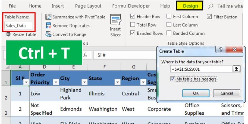
We will store information about products, sales and customers in three tables (on the same sheet or on different ones – it doesn’t matter). It is fundamentally important to turn them into “smart tables” with auto-size, so as not to think about it in the future. This is done with the command Format as a table tab Home (Home — Format as Table). On the tab that then appears Constructor (Design) give tables descriptive names in the field Table name for later use:
In total, we should get three “smart tables”:
Please note that the tables may contain additional clarifying data. So, for example, our Pricecontains additional information about the category (product group, packaging, weight, etc.) of each product, and the table Client — city and region (address, TIN, bank details, etc.) of each of them.
Table Sales will be used by us later to enter completed transactions into it.
Step 2. Create a data entry form
Of course, you can enter sales data directly into the green table Sales, but this is not always convenient and entails the appearance of errors and typos due to the “human factor”. Therefore, it would be better to make a special form for entering data on a separate sheet of something like this:
In cell B3, to get the updated current date-time, use the function The TDATA (NOW). If time is not needed, then instead The TDATA function can be applied TODAY (TODAY).
In cell B11, find the price of the selected product in the third column of the smart table Price using the function VPR (VLOOKUP). If you have not encountered it before, then first read and watch the video here.
In cell B7, we need a dropdown list with products from the price list. For this you can use the command Data – Data Validation (Data — Validation), specify as a constraint List (List) and then enter in the field Source (Source) link to column Name from our smart table Price:
Similarly, a drop-down list with clients is created, but the source will be narrower:
=INDIRECT(“Customers[Client]”)
Function INDIRECT (INDIRECT) is needed, in this case, because Excel, unfortunately, does not understand direct links to smart tables in the Source field. But the same link “wrapped” in a function INDIRECT at the same time, it works with a bang (more about this was in the article about creating drop-down lists with content).
Step 3. Adding a sales entry macro
After filling out the form, you need to add the data entered into it to the end of the table Sales. Using simple links, we will form a line to be added right below the form:
Those. cell A20 will have a link to =B3, cell B20 will have a link to =B7, and so on.
Now let’s add a 2-line elementary macro that copies the generated string and adds it to the Sales table. To do this, press the combination Alt + F11 or button Visual Basic tab developer (Developer). If this tab is not visible, then enable it first in the settings File – Options – Ribbon Setup (File — Options — Customize Ribbon). In the Visual Basic editor window that opens, insert a new empty module through the menu Insert – Module and enter our macro code there:
Sub Add_Sell() Worksheets("Input Form").Range("A20:E20").Copy 'Copy the data line from the form n = Worksheets("Sales").Range("A100000").End(xlUp). Row 'determine the number of the last row in the table. Sales Worksheets("Sales").Cells(n + 1, 1).PasteSpecial Paste:=xlPasteValues 'paste into the next empty line Worksheets("Input Form").Range("B5,B7,B9").ClearContents 'clear end sub form Now we can add a button to our form to run the created macro using the dropdown list Insert tab developer (Developer — Insert — Button):
After you draw it, holding down the left mouse button, Excel will ask you which macro you need to assign to it – select our macro Add_Sell. You can change the text on a button by right-clicking on it and selecting the command Change text.
Now, after filling out the form, you can simply click on our button, and the entered data will be automatically added to the table Sales, and then the form is cleared to enter a new deal.
Step 4 Linking Tables
Before building the report, let’s link our tables together so that later we can quickly calculate sales by region, customer, or category. In older versions of Excel, this would require the use of several functions. VPR (VLOOKUP) for substituting prices, categories, customers, cities, etc. to the table Sales. This requires time and effort from us, and also “eats” a lot of Excel resources. Starting with Excel 2013, everything can be implemented much more simply by setting up relationships between tables.
To do this, on the tab Data (Date) click Relations (Relations). In the window that appears, click the button Create (new) and select from the drop-down lists the tables and column names by which they should be related:
An important point: the tables must be specified in this order, i.e. linked table (Price) must not contain in the key column (Name) duplicate products, as it happens in the table Sales. In other words, the associated table must be one in which you would search for data using VPRif it were used.
Of course, the table is connected in a similar way Sales with table Client by common column Customer:
After setting up the links, the window for managing links can be closed; you do not have to repeat this procedure.
Step 5. We build reports using the summary
Now, to analyze sales and track the dynamics of the process, let’s create, for example, some kind of report using a pivot table. Set active cell to table Sales and select the tab on the ribbon Insert – PivotTable (Insert — Pivot Table). In the window that opens, Excel will ask us about the data source (i.e. table Sales) and a place to upload the report (preferably on a new sheet):
The vital point is that it is necessary to enable the checkbox Add this data to the data model (Add data to Data Model) at the bottom of the window so that Excel understands that we want to build a report not only on the current table, but also use all relationships.
After clicking on OK a panel will appear in the right half of the window Pivot table fieldswhere to click the link Allto see not only the current one, but all the “smart tables” that are in the book at once. And then, as in the classic pivot table, you can simply drag the fields we need from any related tables into the area Filter, Rows, Stolbtsov or Values – and Excel will instantly build any report we need on the sheet:
Do not forget that the pivot table needs to be updated periodically (when the source data changes) by right-clicking on it and selecting the command Update & Save (Refresh), because it cannot do it automatically.
Also, by selecting any cell in the summary and pressing the button Pivot Chart (Pivot Chart) tab Analysis (Analysis) or Parameters (Options) you can quickly visualize the results calculated in it.
Step 6. Fill out the printables
Another typical task of any database is the automatic filling of various printed forms and forms (invoices, invoices, acts, etc.). I already wrote about one of the ways to do this. Here we implement, for example, filling out the form by account number:
It is assumed that in cell C2 the user will enter a number (row number in the table Sales, in fact), and then the data we need is pulled up using the already familiar function VPR (VLOOKUP) and features INDEX (INDEX).
- How to use the VLOOKUP function to look up and lookup values
- How to replace VLOOKUP with INDEX and MATCH functions
- Automatic filling of forms and forms with data from the table
- Creating Reports with PivotTables