Correlation analysis in Excel. An example of performing a correlation analysis

Correlation analysis is a common research method used to determine the level of dependence of the 1st value on the 2nd. The spreadsheet has a special tool that allows you to implement this type of research.

The essence of correlation analysis

It is necessary to determine the relationship between two different quantities. In other words, it reveals in which direction (smaller / larger) the value changes depending on changes in the second.

Purpose of correlation analysis

Dependence is established when the identification of the correlation coefficient begins. This method differs from regression analysis, as there is only one indicator calculated using correlation. The interval changes from +1 to -1. If it is positive, then an increase in the first value contributes to an increase in the 2nd. If negative, then an increase in the 1st value contributes to a decrease in the 2nd. The higher the coefficient, the stronger one value affects the second.

Important! At the 0th coefficient, there is no relationship between the quantities.

Calculation of the correlation coefficient

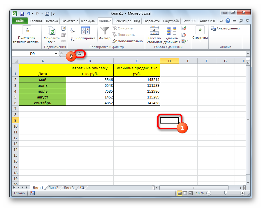
Let’s analyze the calculation on several samples. For example, there is tabular data, where spending on advertising promotion and sales volume are described by months in separate columns. Based on the table, we will find out the level of dependence of sales volume on the money spent on advertising promotion.

Method 1: Determining Correlation Through the Function Wizard

CORREL – a function that allows you to implement a correlation analysis. General form – CORREL(massiv1;massiv2). Detailed instructions:

1. It is necessary to select the cell in which it is planned to display the result of the calculation. Click “Insert Function” located to the left of the text field to enter the formula.

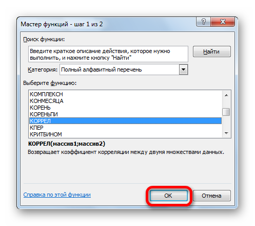
2. The Function Wizard opens. Here you need to find CORREL, click on it, then on “OK”.

3. The arguments window opens. In the line “Array1” you must enter the coordinates of the intervals of the 1st of the values. In this example, this is the Sales Value column. You just need to select all the cells that are in this column. Similarly, you need to add the coordinates of the second column to the “Array2” line. In our example, this is the Advertising Costs column.

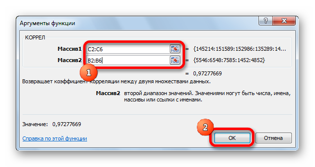
4. After entering all the ranges, click on the “OK” button.

The coefficient was displayed in the cell that was indicated at the beginning of our actions. The result obtained is 0,97. This indicator reflects the high dependence of the first value on the second.

Method 2: Calculate Correlation Using the Analysis ToolPak

There is another method for determining correlation. Here one of the functions found in the analysis package is used. Before using it, you need to activate the tool. Detailed instructions:

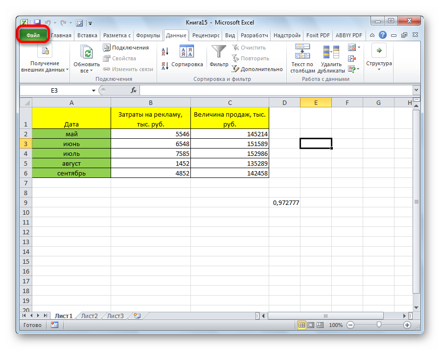
1. Go to the “File” section.

2. A new window will open, in which you need to click on the “Settings” section.
3. Click on “Add-ons”.
4. We find the element “Management” at the bottom. Here you need to select “Excel Add-ins” from the context menu and click “OK”.

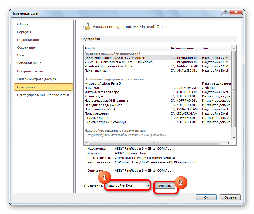
5. A special add-ons window has opened. Place a checkmark next to the “Analysis Package” element. We click “OK”.
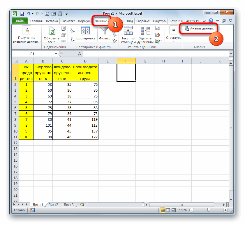
6. Activation was successful. Now let’s go to Data. The “Analysis” block appeared, in which you need to click “Data Analysis”.
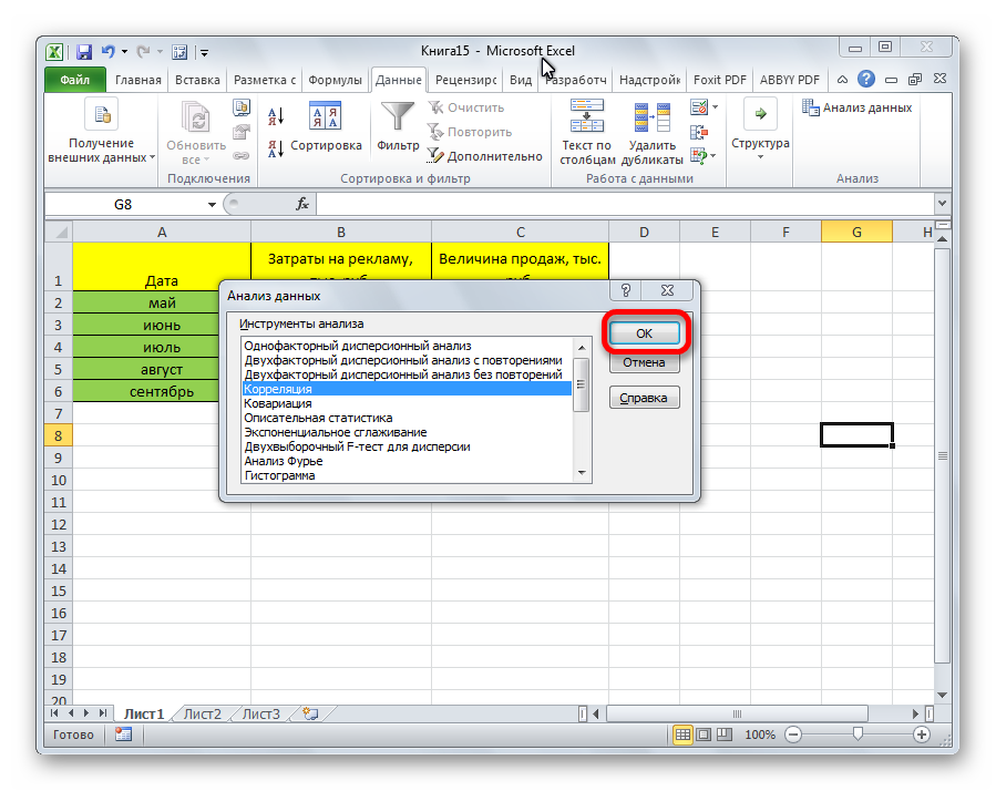
7. In the new window that appears, select the “Correlation” element and click on “OK”.

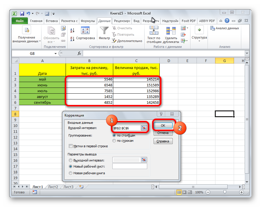
8. The analysis settings window appeared on the screen. In the line “Input interval” it is necessary to enter the range of absolutely all columns taking part in the analysis. In this example, these are the columns “Sales value” and “Advertising costs”. The output display settings are initially set to New Worksheet, which means that the results will be displayed on a different sheet. Optionally, you can change the output location of the result. After making all the settings, click on “OK”.

The final scores are out. The result is the same as in the first method – 0,97.

Definition and calculation of multiple correlation coefficient in MS Excel

To identify the level of dependence of several quantities, multiple coefficients are used. In the future, the results are summarized in a separate table, called the correlation matrix.

Detailed guide:

1. In the “Data” section, we find the already known “Analysis” block and click “Data Analysis”.

2. In the window that appears, click on the “Correlation” element and click on “OK”.
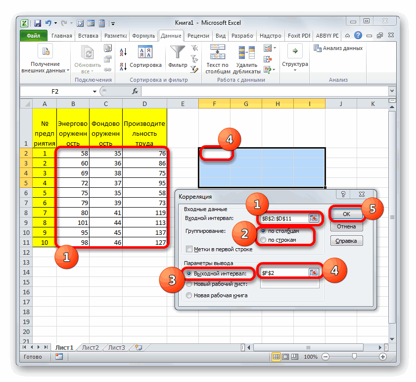
3. In the line “Input interval” we drive in the interval for three or more columns of the source table. The range can be entered manually or simply select it with the LMB, and it will automatically appear in the desired line. In “Grouping” select the appropriate grouping method. In “Output Parameter” specifies the location where the correlation results will be displayed. We click “OK”.

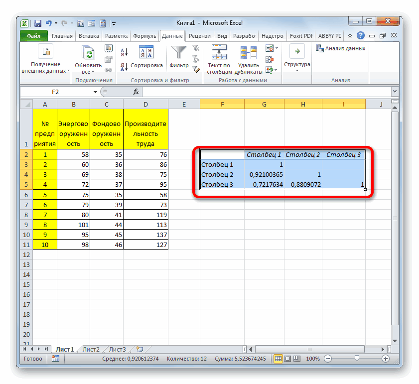
4. Ready! The correlation matrix was built.

Pair Correlation Coefficient in Excel

Let’s figure out how to correctly draw the pair correlation coefficient in an Excel spreadsheet.

Calculation of pair correlation coefficient in Excel

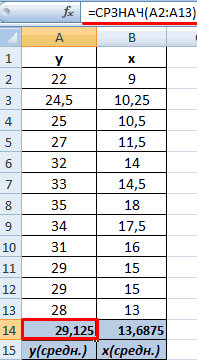
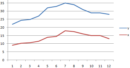
For example, you have x and y values.

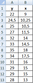
X is the dependent variable and y is the independent. It is necessary to find the direction and strength of the relationship between these indicators. Step-by-step instruction:

1. Let’s find the average values ​​using the function HEART.

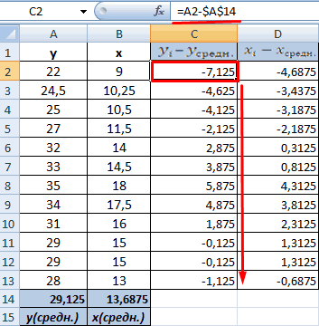
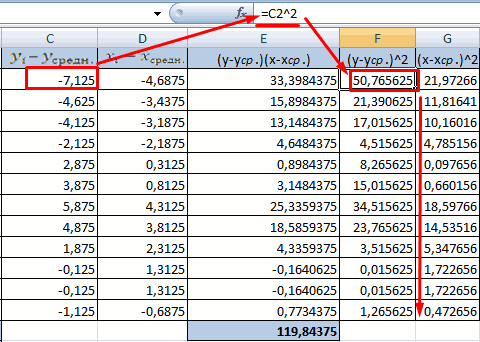
2. Let’s calculate each х и xavg, у и avg using the «-» operator.

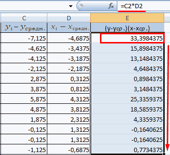
3. We multiply the calculated differences.

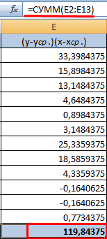
4. We calculate the sum of the indicators in this column. The numerator is the result found.

5. Calculate the denominators of the difference х и x-average, y и y-medium. To do this, we will perform the squaring.

6. Using the function AUTOSUMMA, find the indicators in the resulting columns. We do multiplication. Using the function ROOT square the result.

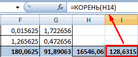
7. We calculate the quotient using the values ​​​​of the denominator and numerator.

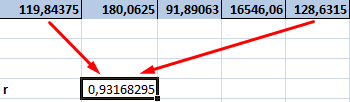
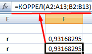
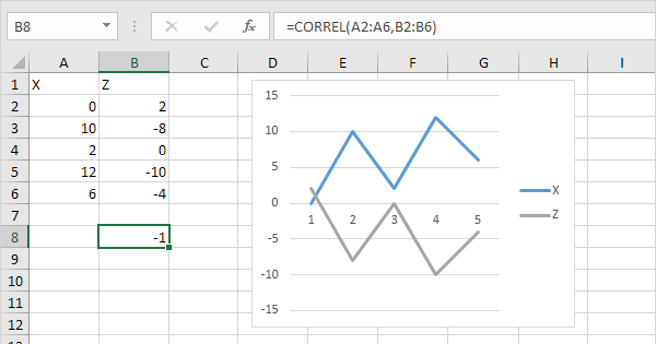
8. CORREL is an integrated function that allows you to prevent complex calculations. We go to the “Function Wizard”, select CORREL and specify the arrays of indicators х и у. We build a graph that displays the obtained values.

Matrix of Pairwise Correlation Coefficients in Excel

Let’s analyze how to calculate the coefficients of paired matrices. For example, there is a matrix of four variables.

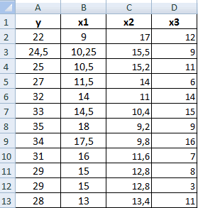
Step-by-step instruction:

1. We go to the “Data Analysis”, located in the “Analysis” block of the “Data” tab. Select Correlation from the list that appears.
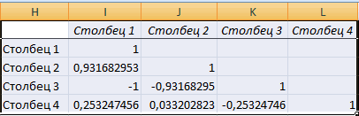
2. We set all the necessary settings. “Input interval” – the interval of all four columns. “Output interval” – the place where we want to display the totals. We click on the “OK” button.
3. A correlation matrix was built in the chosen place. Each intersection of a row and a column is a correlation coefficient. The number 1 is displayed when the coordinates match.

CORREL function to determine relationship and correlation in Excel

CORREL – a function used to calculate the correlation coefficient between 2 arrays. Let’s look at four examples of all the abilities of this function.

Examples of using the CORREL function in Excel

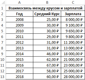
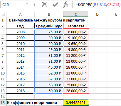
First example. There is a plate with information about the average salaries of the company’s employees over the course of eleven years and the exchange rate of $. It is necessary to identify the relationship between these two quantities. The table looks like this:

The calculation algorithm looks like this:

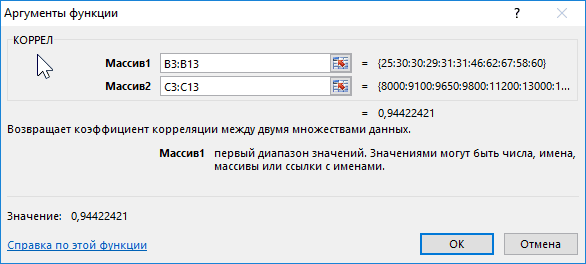
The displayed score is close to 1. Result:

Determination of the correlation coefficient of the impact of actions on the result

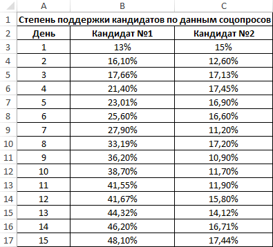
Second example. Two bidders approached two different agencies for help with a fifteen-day promotion. Every day a social poll was conducted, which determined the degree of support for each applicant. Any interviewee could choose one of the two applicants or oppose all. It is necessary to determine how much each advertising promotion influenced the degree of support for applicants, which company is more efficient.

Using the formulas below, we calculate the correlation coefficient:

• =CORREL(A3:A17;B3:B17).
• =CORREL(A3:A17;C3:C17).

Results:

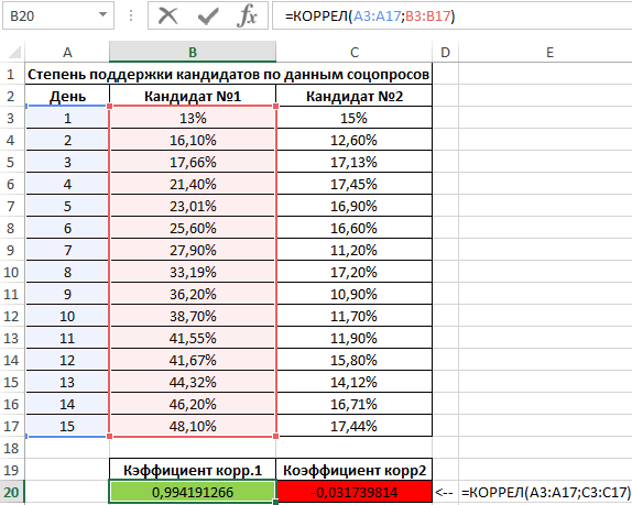
From the results obtained, it becomes clear that the degree of support for the 1st applicant increased with each day of advertising promotion, therefore, the correlation coefficient approaches 1. When advertising was launched, the other applicant had a large number of trust, and for 5 days there was a positive trend. Then the degree of trust decreased and by the fifteenth day it dropped below the initial indicators. Low scores suggest that promotion has negatively impacted support. Do not forget that other concomitant factors that are not considered in tabular form could also affect the indicators.

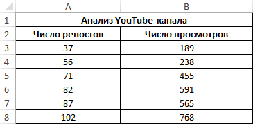
Analysis of content popularity by correlation of video views and reposts

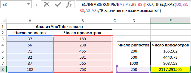
Third example. A person to promote their own videos on YouTube video hosting uses social networks to advertise the channel. He notices that there is some relationship between the number of reposts in social networks and the number of views on the channel. Is it possible to predict future performance using spreadsheet tools? It is necessary to identify the reasonableness of applying the linear regression equation to predict the number of video views depending on the number of reposts. Table with values:

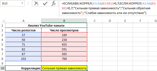
Now it is necessary to determine the presence of a relationship between 2 indicators according to the formula below:

0,7;IF(CORREL(A3:A8;B3:B8)>0,7;”Strong direct relationship”;”Strong inverse relationship”);”Weak or no relationship”)’ class=’formula’>

If the resulting coefficient is higher than 0,7, then it is more appropriate to use the linear regression function. In this example, we do:

Now we are building a graph:

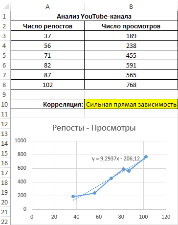
We apply this equation to determine the number of views at 200, 500 and 1000 shares: =9,2937*D4-206,12. We get the following results:

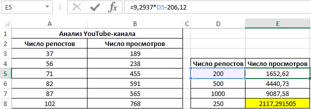
Function FORECAST allows you to determine the number of views at the moment, if there were, for example, two hundred and fifty reposts. We apply: 0,7;PREDICTION(D7;B3:B8;A3:A8);”The values ​​are not related”)’ class=’formula’>. We get the following results:

Features of using the CORREL function in Excel

This function has the following features:

1. Empty cells are not taken into account.
2. Cells containing Boolean and Text type information are not taken into account.
3. Double negation “-” is used to account for logical values ​​in the form of numbers.
4. The number of cells in the studied arrays must match, otherwise the #N/A message will be displayed.

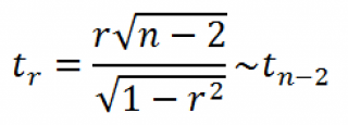
Assessment of the statistical significance of the correlation coefficient

When testing the significance of a correlation coefficient, the null hypothesis is that the indicator has a value of 0, while the alternative does not. The following formula is used for verification:

Conclusion

Correlation analysis in a spreadsheet is a simple and automated process. To perform it, you only need to know where the necessary tools are located and how to activate them through the program settings.