Chart by selected cell

Suppose that you and I need to visualize data from the following table with car sales values ​​​​by different countries in 2021 (real data taken from here, by the way):

Since the number of data series (countries) is large, trying to cram all of them into one graph at once will either lead to a terrible “spaghetti chart” or to building separate charts for each series, which is very cumbersome.

An elegant solution to this problem can be to plot a chart only on the data from the current row, i.e. the row where the active cell is located:

Implementing this is very easy – you only need two formulas and one tiny macro in 3 lines.

Step 1. Current line number

The first thing we need is a named range that calculates the row number on the sheet where our active cell is now located. Opening on a tab Formulas – Name Manager (Formulas — Name manager), click on the button Create (Create) and enter the following structure there:

Step 2. Link to the title

To display the selected country in the title and legend of the chart, we need to get a reference to the cell with its (country) name from the first column. To do this, we create another local (i.e. Area = current sheet, not Book!) a named range with the following formula:

Here, the INDEX function selects from a given range (column A, where our signing countries lie) a cell with the row number that we previously determined.

Step 3. Link to data

Now, in a similar way, let’s get a link to a range with all the sales data from the current row, where the active cell is now located. Create another named range with the following formula:

Here, the third argument, which is zero, causes INDEX to return not a single value, but the entire row as a result.

Step 4. Substituting Links in the Chart

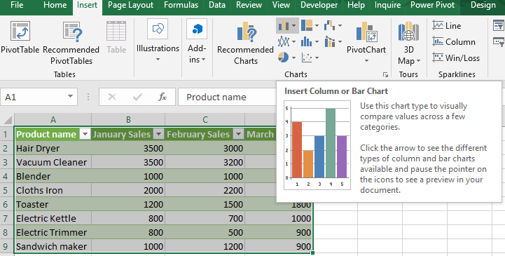
Now select the table header and the first row with data (range) and build a chart based on them using Insert – Charts (Insert — Charts). If you select a row with data in the chart, then the function will be displayed in the formula bar ROW (SERIES) is a special function that Excel automatically uses when creating any chart to refer to the original data and labels:

Let’s carefully replace the first (signature) and third (data) arguments in this function with the names of our ranges from steps 2 and 3:

The chart will start displaying sales data from the current row.

Step 5. Recalculation Macro

The final touch remains. Microsoft Excel recalculates formulas only when the data on the sheet changes or when a key is pressed F9, and we want the recalculation to occur when the selection changes, i.e. when the active cell is moved across the sheet. To do this, we need to add a simple macro to our workbook.

Right-click on the data sheet tab and select the command Source (Source code). In the window that opens, enter the code of the macro-handler for the selection change event:

As you can easily imagine, all it does is trigger a sheet recalculation whenever the position of the active cell changes.

Step 6. Highlighting the Current Line

For clarity, you can also add a conditional formatting rule to highlight the country that is currently displayed on the chart. To do this, select the table and select Home — Conditional Formatting — Create Rule — Use Formula to Determine Cells to Format (Home — Conditional formatting — New rule — Use a formula to determine which cells to format):

Here the formula checks for each cell in the table that its row number matches the number stored in the TekRow variable, and if there is a match, then the fill with the selected color is triggered.

That’s it – simple and beautiful, right?

Notes

• On large tables, all this beauty can slow down – conditional formatting is a resource-intensive thing, and recalculation for each selection can also be heavy.
• To prevent data from disappearing on the chart when a cell is accidentally selected above or below the table, you can add an additional check to the TekRow name using nested IF functions of the form:

  =IF(CELL(“row”)<4,IF(CELL("row")>4,CELL(“row”)))
  

• Highlighting specified columns in a chart
• How to create an interactive chart in Excel
• Coordinate Selection