


Contents
Student’s criterion is a generalized name for a group of statistical tests (usually, the Latin letter “t” is added before the word “criterion”). It is most often used to check if the means of two samples are equal. Let’s see how to calculate this criterion in Excel using a special function.
Student’s t-test calculation
In order to perform the corresponding calculations, we need a function “STUDENT TEST”, in earlier versions of Excel (2007 and older) – “TTEST”, which is also in modern editions to maintain compatibility with older documents.
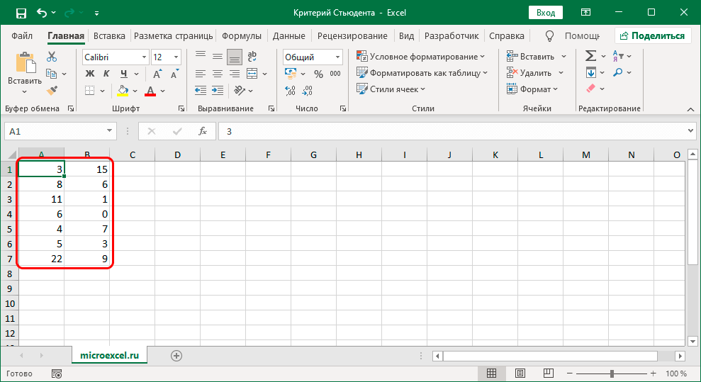
The function can be used in different ways. Let’s analyze each option separately using the example of a table with two rows-columns of numerical values.
Method 1: Using the Function Wizard
This method is good because you do not need to remember the formula of the function (the list of its arguments). So, the algorithm of actions is as follows:
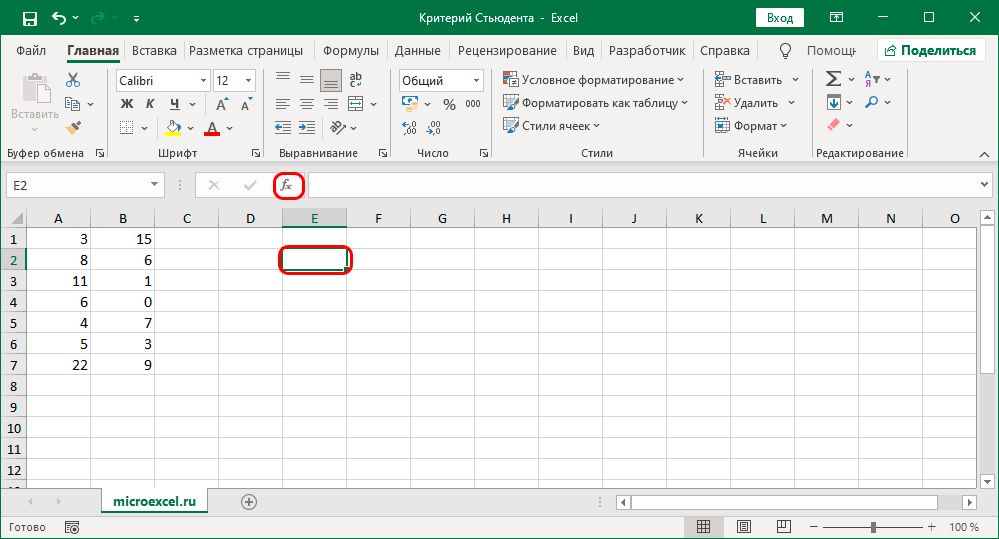
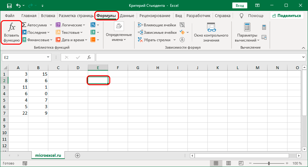
- We stand in any free cell, then click on the icon “Insert function” to the left of the formula bar.

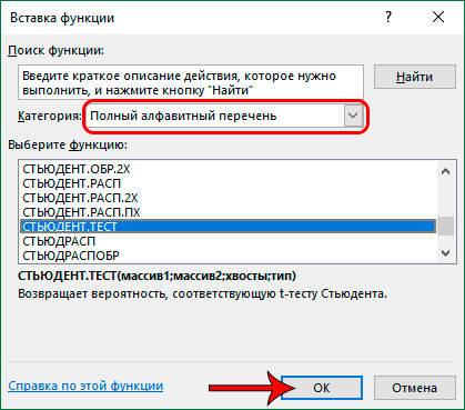
- In the opened window Function Wizards choose a category “Full alphabetical list”, in the list below we find the operator “STUDENT TEST”, mark it and click OK.
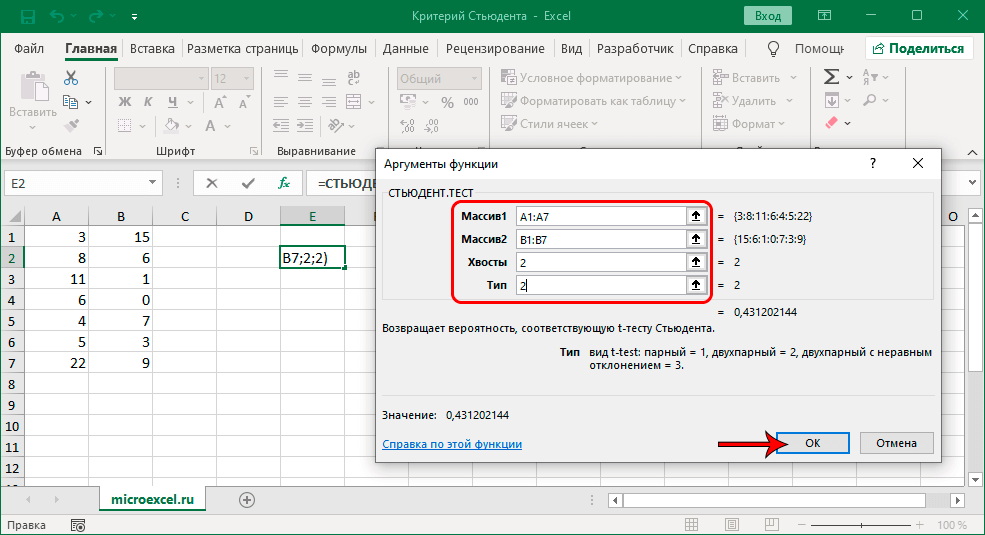
- A window will appear on the screen in which we fill in the arguments of the function, after which we press OK:
- “Massiv1“And “Massive2” – specify the ranges of cells containing series of numbers (in our case, this is “A2:A7” и “B2:B7”). We can do this manually by entering the coordinates from the keyboard, or simply select the desired elements in the table itself.
- “Tails” – I write a number “1”if you want to perform a one-way distribution calculation, or “2” – for double-sided.
- “Tip” – in this field indicate: “1” – if the sample consists of dependent variables; “2” – from independent; “3” – from independent values with unequal deviation.
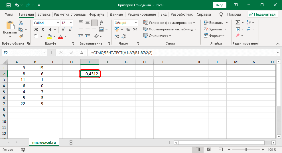
- As a result, the calculated value of the criterion will appear in our cell with the function.
Method 2: insert a function through “Formulas”
- Switch to tab “Formulas”, which also has a button “Insert function”, which is what we need.
- As a result, it will open Function wizard, further actions in which are similar to those described above.
Via tab “Formulas” function “STUDENT TEST” can be run differently:
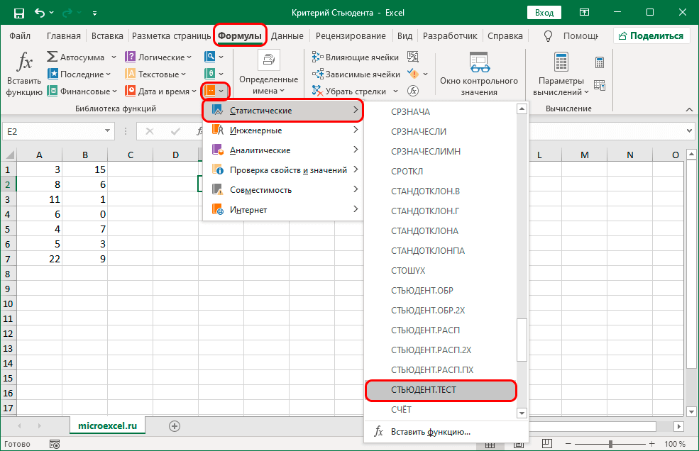
- In the tool group “Function Library” click on the icon “Other Features”, after which a list will open, in which we select a section “Statistical”. By scrolling through the proposed list, we can find the operator we need.
- The screen will display the window for filling in the arguments, which we have already met earlier.
Method 3: Entering the formula manually
Experienced users can do without Function Wizards and in the required cell immediately enter a formula with links to the desired data ranges and other parameters. The function syntax in general looks like this:
= STUDENT.TEST(Array1;Array2;Tails;Type)
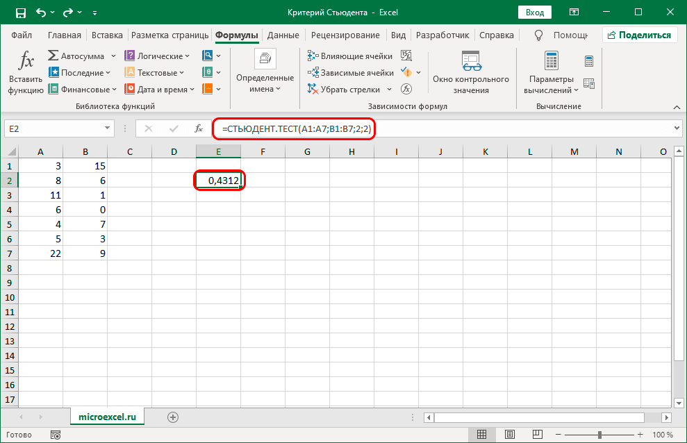
We have analyzed each of the arguments in the first section of the publication. All that remains to be done after typing the formula is to press Enter to perform the calculation.
Conclusion
Thus, you can calculate the Student’s t-test in Excel using a special function that can be launched in different ways. Also, the user has the opportunity to immediately enter the function formula in the desired cell, however, in this case, you will have to remember its syntax, which can be troublesome due to the fact that it is not used so often.