


Excel has made calculating the average of multiple cells a very easy task – just use the function AVERAGE (AVERAGE). But what if some values carry more weight than others? For example, in many courses, tests carry more weight than assignments. For such cases, it is necessary to calculate weighted average.
Excel does not have a function for calculating the weighted average, but there is a function that will do most of the work for you: SUMPRODUCT (SUM PRODUCT). And even if you’ve never used this feature before, by the end of this article you’ll be using it like a pro. The method we use works in any version of Excel as well as other spreadsheets such as Google Sheets.
We prepare the table
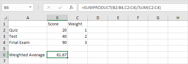
If you are going to calculate a weighted average, you will need at least two columns. The first column (column B in our example) contains the scores for each assignment or test. The second column (column C) contains the weights. More weight means more influence of the task or test on the final grade.
To understand what weight is, you can think of it as a percentage of your final grade. In fact, this is not the case, since in this case the weights should add up to 100%. The formula that we will analyze in this lesson will calculate everything correctly and does not depend on the amount that the weights add up to.
We enter the formula
Now that our table is ready, we add the formula to the cell B10 (any empty cell will do). As with any other formula in Excel, we start with an equal sign (=).
The first part of our formula is the function SUMPRODUCT (SUM PRODUCT). Arguments must be enclosed in brackets, so we open them:
=СУММПРОИЗВ(
=SUMPRODUCT(
Next, add the function arguments. SUMPRODUCT (SUMPRODUCT) can have multiple arguments, but usually two are used. In our example, the first argument will be a range of cells. B2: B9A that contains the scores.
=СУММПРОИЗВ(B2:B9
=SUMPRODUCT(B2:B9
The second argument will be a range of cells C2: C9, which contains the weights. These arguments must be separated by a semicolon (comma). When everything is ready, close the brackets:
=СУММПРОИЗВ(B2:B9;C2:C9)
=SUMPRODUCT(B2:B9,C2:C9)
Now let’s add the second part of our formula, which will divide the result calculated by the function SUMPRODUCT (SUMPRODUCT) by the sum of the weights. We will discuss later why this is important.
To perform the division operation, we continue the already entered formula with the symbol / (straight slash), and then write the function SUM (SUM):
=СУММПРОИЗВ(B2:B9;C2:C9)/СУММ(
=SUMPRODUCT(B2:B9, C2:C9)/SUM(
For function SUM (SUM) we will specify only one argument – a range of cells C2: C9. Don’t forget to close the parentheses after entering the argument:
=СУММПРОИЗВ(B2:B9;C2:C9)/СУММ(C2:C9)
=SUMPRODUCT(B2:B9, C2:C9)/SUM(C2:C9)
Ready! After pressing the key Enter, Excel will calculate the weighted average. In our example, the final result will be 83,6.
How it works
Let’s break down each part of the formula, starting with the function SUMPRODUCT (SUMPRODUCT) to understand how it works. Function SUMPRODUCT (SUMPRODUCT) calculates the product of each item’s score and its weight, and then sums all the resulting products. In other words, the function finds the sum of the products, hence the name. So for Assignments 1 multiply 85 by 5, and for The test multiply 83 by 25.
If you’re wondering why we need to multiply the values in the first part, imagine that the greater the weight of the task, the more times we have to consider the grade for it. For example, Task 2 counted 5 times and Final exam – 45 times. That’s why Final exam has a greater impact on the final grade.
For comparison, when calculating the usual arithmetic mean, each value is taken into account only once, that is, all values have equal weight.
If you could look under the hood of a function SUMPRODUCT (SUMPRODUCT), we saw that in fact she believes this:
=(B2*C2)+(B3*C3)+(B4*C4)+(B5*C5)+(B6*C6)+(B7*C7)+(B8*C8)+(B9*C9)
Luckily, we don’t need to write such a long formula because SUMPRODUCT (SUMPRODUCT) does all this automatically.
A function in itself SUMPRODUCT (SUMPRODUCT) returns us a huge number − 10450. At this point, the second part of the formula comes into play: /SUM(C2:C9) or /SUM(C2:C9), which returns the result to the normal range of scores, giving the answer 83,6.
The second part of the formula is very important because allows you to automatically correct calculations. Remember that weights don’t have to add up to 100%? All this thanks to the second part of the formula. For example, if we increase one or more weight values, the second part of the formula will simply divide by the larger value, again resulting in the correct answer. Or we can make the weights much smaller, for example by specifying values like 0,5, 2,5, 3 or 4,5, and the formula will still work correctly. It’s great, right?