


This simple technique is useful to anyone who has ever made a report in their life, where you need to visually show the change in any parameter (prices, profits, expenses) compared to previous periods. Its essence is that right inside the cells, you can add green and red arrows to show where the original value has moved:

There are several ways to implement this.
Method 1. Custom format with special characters
Suppose we have such a table with the initial data that we need to visualize:

To calculate percentage movements in cell D4, a simple formula is used that calculates the difference between this year’s and last year’s prices and the percentage format of the cells. To add fancy arrows to cells, do the following:
Select any empty cell and enter the triangle up and triangle down symbols into it using the command Insert – Symbol (Insert — Symbol):

It is better to use standard fonts (Arial, Tahoma, Verdana), which are definitely available on any computer. Close the insert window, select both entered characters (in the formula bar, not the cell with them!) and copy to Clipboard (Ctrl + C).
Select cells with percentages (D4:D10) and open the window Cell Format (can be used Ctrl + 1). On the tab Number (number) select a format from the list All formats (Custom) and paste the copied characters into the string A type, and then manually add zeros and percentages to them from the keyboard to get the following:

The principle is simple: if there is a positive number in the cell, then the first custom format will be applied to it, if negative – the second. There is a mandatory separator between the formats – a semicolon. And in no case do not insert any spaces “for beauty”. After clicking on OK our table will look almost as intended:

There are two ways to add red and green color to cells. The first is to return to the window Cell format and add the desired colors in square brackets right in our custom format:

Personally, I don’t really like the poisonous green that results in this case, so I prefer the second option – add color using conditional formatting. To do this, select the cells with percentages and select on the tab Home — Conditional Formatting — Cell Selection Rules — More (Home — Conditional formatting — Highlight Cell Rules — Greater Then), enter 0 as the threshold value, and set the desired color:

Then repeat these steps for negative values, choosing Less (Less Then)to format them green.
If you experiment a little with symbols, you can find many similar options for implementing a similar trick with other symbols:

Method 2: Conditional formatting
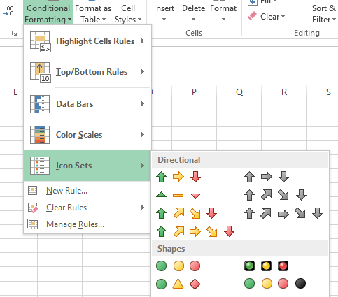
Select the cells with percentages and open on the tab Home — Conditional Formatting — Icon Sets — Other Rules (Home — Conditional formatting — Icon Sets — More). In the window that opens, select the necessary icons from the drop-down lists and set restrictions for substituting each of them as in the figure:

After clicking on OK we get the result:

The advantages of this method are its relative simplicity and a decent set of various built-in icons that you can use:

The downside is that this set does not, for example, have a red up arrow and a green down arrow, i.e. it would be logical to use these icons for profit growth, but not so much for price growth. But, in any case, this method also deserves to be known to you 😉
- Video tutorial on conditional formatting in Excel
- How to create custom custom cell formats in Excel (thousand roubles, pcs., people. etc.)
- How to build a Plan-Fact chart