


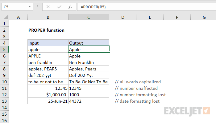
When you think of Excel functions, you most likely think of some kind of calculation or number operation. Yes, indeed, with the help of Excel functions, you can perform many different operations, but, in addition, some functions can also help you format text. A good example is the function PROPNACH (PROPER), which capitalizes the first letter of every word in the cell.
If you have cells containing names or titles, you can use the function PROPNACHto make sure all words are capitalized. Function PROPNACH works in Google Sheets too. Let’s imagine that your company wants to reward someone for merit. You asked colleagues to fill in the table with the names of those employees who, in their opinion, deserve an award.
Unfortunately, not all the names of the nominees are capitalized, so the table does not look neat. Of course, you can go through the entire column and correct the names manually, but it will be faster, easier and more correct to use the function PROPNACH.
In this example, the names of the nominees are in column A, so we will write the formula in column B. In cell B2 enter an expression that will tell Excel to take the words from the cell A2 and capitalize them. The formula will look like this:
=PROPER(A2)
=ПРОПНАЧ(A2)
Most likely, you remember from the lesson on simple formulas in our Excel 2013 tutorial that it is important not to forget to start all formulas with an equal sign (=).
Once the formula has been entered, press Enter. In a cell B2 the name from the cell will be displayed A2capitalized: Thomas Lynley.
All we have to do is copy the formula to the rest of the cells. To do this, select the cell with the formula and, using the autofill marker, copy the formula to 14 strings. Column B will display a list of names with correct capitalization:
Excellent! Now in our table all the names of the nominees are spelled correctly, i.e. with a capital letter. There’s one more problem: Column A still contains lowercase names. We can’t just delete column A because it is referenced by the formulas in column B. Let’s do it differently – copy the values from column B to a new column using the tool Paste Values (Insert values).
To do this, select the cells B2: B14 and press command Copy (Copy), or use the keyboard shortcut Ctrl + C on keyboard. Right-click on the cell where you want to paste the copied values and in the context menu that appears, select Values (Values).
If you are working in Google Sheets: right-click, select Paste special (Paste Special) and then Paste values only (Insert values only).
Now we have a column with correctly spelled names and, moreover, not dependent on any formulas or cell references. This means that we can remove our auxiliary columns (columns A and B). The result is a nice and neat table, in which each name of the nominee is written with a capital letter.