Transposing a table in Excel

Surely every user working in Excel has come across a situation where the rows and columns of a table need to be swapped. If we are talking about a small amount of data, then the procedure can be performed manually, and in other cases, when there is a lot of information, special tools will be very useful or even indispensable, with which you can automatically turn the table. Let’s see how it’s done.

Table transposition

Transposition – this is the “transfer” of the rows and columns of the table in places. This operation can be performed in different ways.

Method 1: Use Paste Special

This method is used most often, and here is what it consists of:

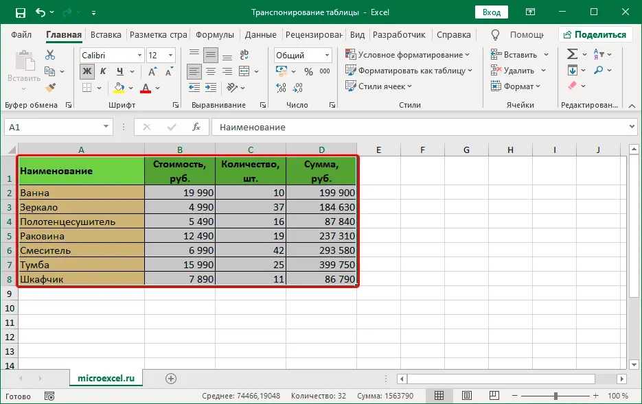
1. Select the table in any convenient way (for example, by holding down the left mouse button from the top left cell to the bottom right).
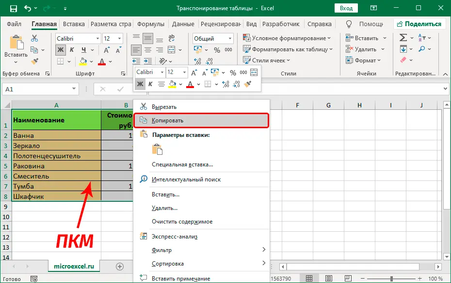
2. Now right-click on the selected area and select the command from the context menu that opens. “Copy” (or instead just press the combination Ctrl + C).
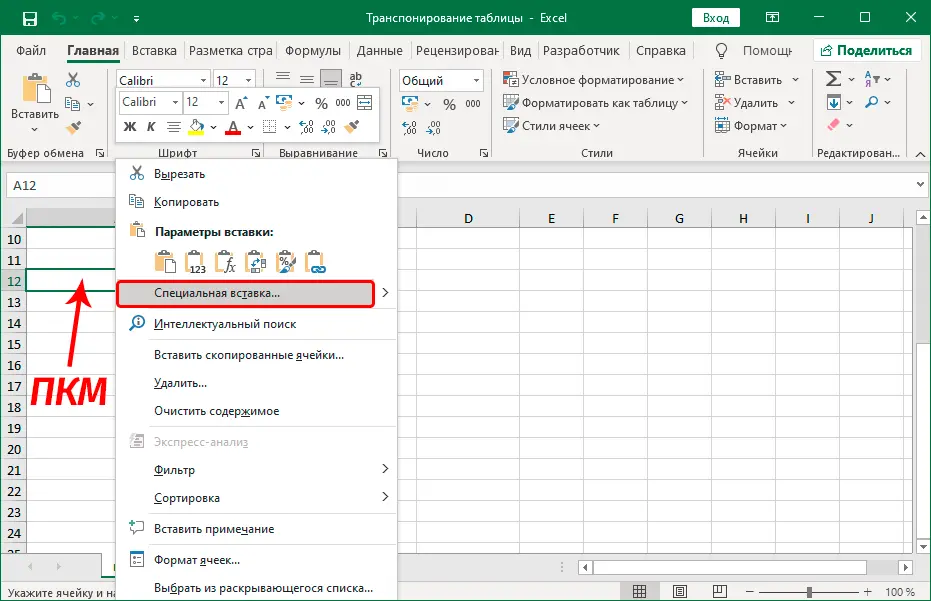
3. On the same or on another sheet, we stand in the cell, which will become the top left cell of the transposed table. We right-click on it, and this time we need the command in the context menu “Special Paste”.
4. In the window that opens, check the box next to “Transpose” and click OK.
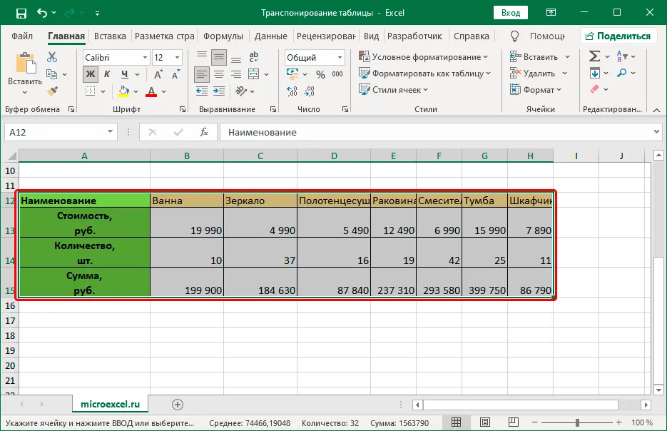
5. As we can see, an automatically inverted table appeared in the selected place, in which the columns of the original table became rows and vice versa. Now we can start customizing the appearance of the data to our liking. If the original table is no longer needed, it can be deleted.

Method 2: Apply the “TRANSPOSE” Function

To flip a table in Excel, you can use a special function “TRANSP”.

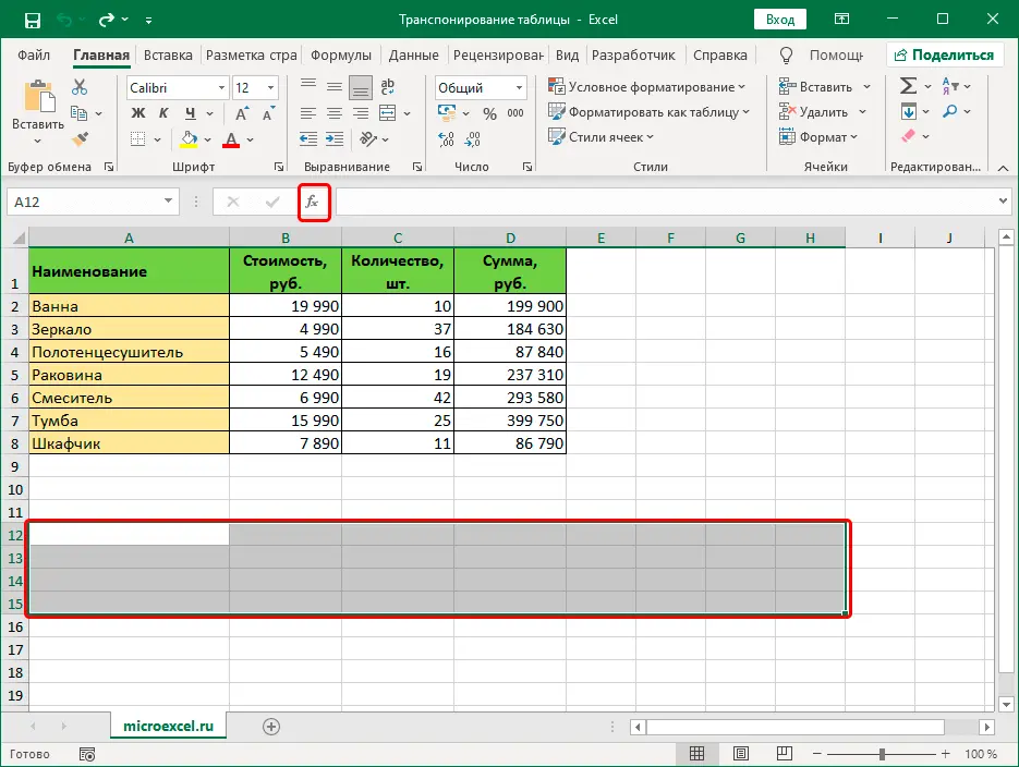
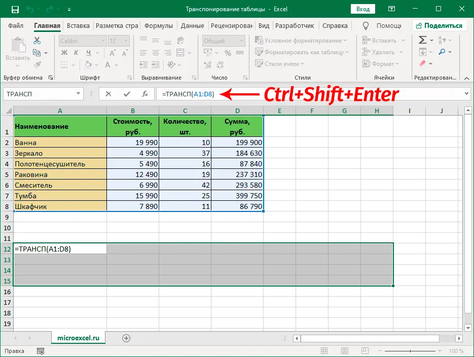
1. On the sheet, select a range of cells that contains as many rows as there are columns in the original table, and accordingly, the same applies to the columns. Then press the button “Insert function” to the left of the formula bar.
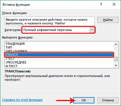
2. In the opened Function Wizard choose a category “Full alphabetical list”, we find the operator “TRANSP”, mark it and click OK.
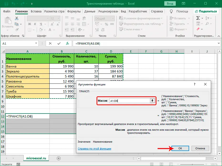
3. The function arguments window will appear on the screen, where you need to specify the coordinates of the table, on the basis of which the transposition will be performed. You can do this manually (keyboard entry) or by selecting a range of cells on a sheet. When everything is ready, click OK.
4. We get this result on the sheet, but that’s not all.
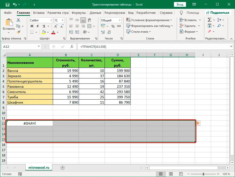
5. Now, in order for the transposed table to appear instead of the error, click on the formula bar to start editing its contents, put the cursor at the very end, and then press the key combination Ctrl + Shift + Enter.
6. Thus, we were able to successfully transpose the original table. In the formula bar, we see that the expression is now framed by curly braces.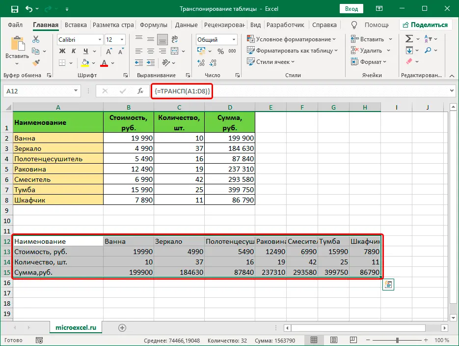Note: Unlike the first method, the primary formatting has not been preserved here, which in some cases is even good, since we can set everything up from scratch the way we want. Also, here we do not have the opportunity to delete the original table, since the function “pulls” the data from it. But the undoubted advantage is that the tables are connected, i.e. any changes to the original data will be immediately reflected in the transposed ones.

Conclusion

Thus, there are two ways that you can use to transpose a table in Excel. Both of them are easy to implement, and the choice of one or another option depends on further plans for working with the initial and received data.