Contents
Excel is a very functional program. It can be used to solve a huge layer of problems that one has to face in business. One of the most common is transportation. Imagine that we need to understand which method of transportation from the manufacturer to the final buyer is the most optimal in terms of time, money and other resources. This problem is quite popular, no matter what industry the business is in. Therefore, let’s take a closer look at how to implement it using Excel.
Description of the transport task
So, we have two counterparties that constantly interact with each other. In our case, this is a buyer and a seller. We need to figure out how to transport goods in such a way that costs are minimal. To do this, you need to present all the data in a schematic or matrix form. In Excel, we use the latter option. In general, there are two types of transport tasks:
- Closed. In this case, supply and demand are in balance.
- Open. There is no equality between supply and demand here. To obtain a solution to this problem, you must first bring it to the first type, equalizing supply and demand. To do this, you need to introduce an additional indicator – the presence of a conditional buyer or seller. In addition, you need to make certain changes to the cost table.
How to enable the Find Solution feature in Excel
To solve transportation problems in Excel, there is a special function called “Search for a solution”. It is not enabled by default, so you need to do the following steps:
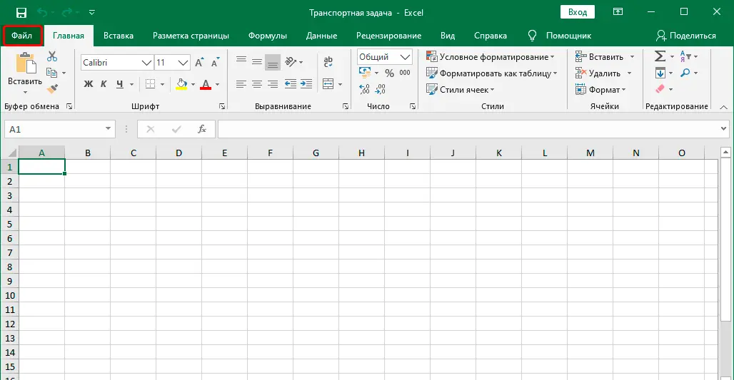
- Open the “File” menu, which is located in the upper left corner of the program window.

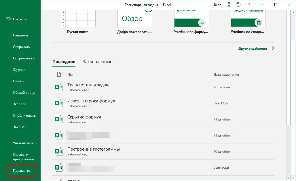
- After that, click on the button with the parameters.

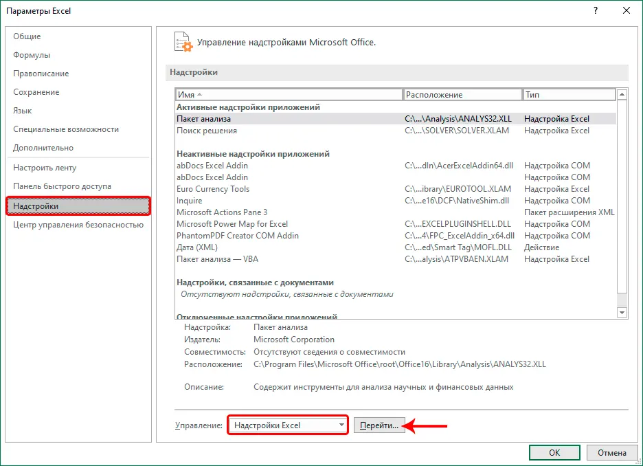
- Next, we find the “Settings” subsection and go to the add-ons management menu. These are small programs that run within the Microsoft Excel environment. We see that at first we clicked on the “Add-ins” menu, and then in the lower right part we set the “Excel Add-ins” item and clicked on the “Go” button. All the necessary actions are highlighted with red rectangles and arrows.

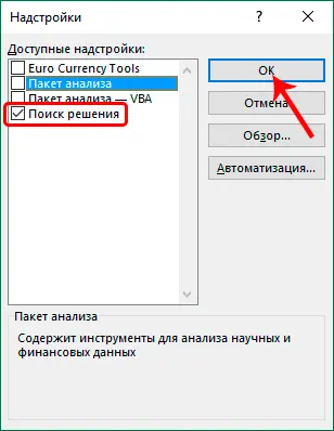
- Next, turn on the add-in “Search for a solution”, after which we confirm our actions by pressing the OK button. Based on the description of the setting, we can see that it is designed to analyze complex data, such as scientific and financial.

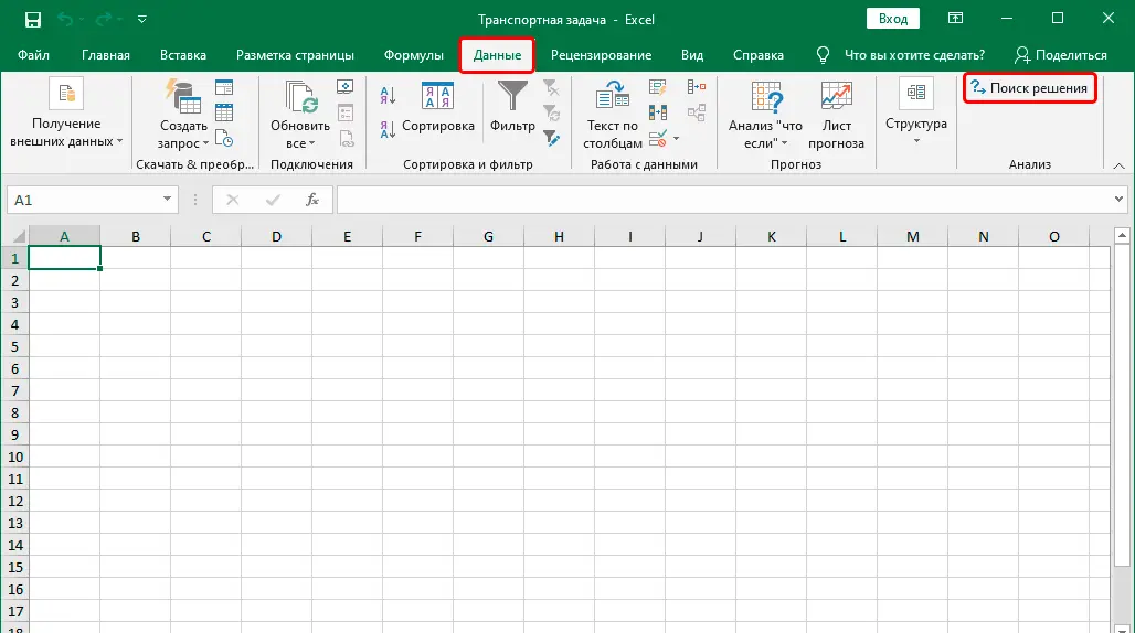
- After that, go to the “Data” tab, where we see a new button, which is called the same as the add-in. It can be found in the Analysis tool group.

It remains only to click on this button, and we proceed to the solution of the transport problem. But before that, we should talk a little more about the Solver tool in Excel. This is a special Excel add-on that makes it possible to find the fastest solution to a problem. A characteristic feature is the consideration of restrictions that the user sets at the preparation stage. In simple terms, this is a subroutine that makes it possible to determine the best way to achieve a certain task. Such tasks may include the following:
- Investing, loading a warehouse or any other similar activity. Including the delivery of goods.
- The best way. This includes objectives such as achieving maximum profit at minimum cost, how to achieve the best quality with available resources, and so on.
In addition to transport tasks, this add-on is also used for the following purposes:
- Development of a production plan. That is, how many units of a product need to be produced in order to achieve maximum income.
- Find the distribution of labor for different types of work so that the total cost of producing a product or service is the smallest.
- Set the minimum time it will take to complete all the work.
As you can see, the tasks are very different. The universal rule for applying this add-in is that before solving the problem, it is necessary to create a model that would correspond to the key characteristics of the problem posed. A model is a collection of functions that use variables as their arguments. That is, values that can change.
It is important to note that the optimization of a set of values is carried out exclusively on one indicator, which is called the objective function.
The Solver add-in enumerates the different values of the variables that are passed to the objective function in such a way that it is the maximum, minimum, or equal to a certain value (this is precisely the restriction). There is another function that is somewhat similar in its principle of operation, and which is often confused with the “Search for a solution”. It’s called “Option Selection”. But if you dig deeper, the difference between them is enormous:
- The Goal Seek function does not work with more than one variable.
- It does not provide for the ability to set limits on variables.
- It is able to determine only the equality of the objective function to a certain value, but does not make it possible to find the maximum and minimum. Therefore, it is not suitable for our task.
- Able to efficiently calculate only if model linear type. If the model is non-linear, then it finds the value that is closest to the original value.
The transport task is much more complicated in its structure, so the “Parameter selection” add-on is not enough for this. Let’s take a closer look at how to implement the “Search for a Solution” function in practice using the example of a transport problem.
An example of solving a transport problem in Excel
In order to clearly demonstrate how to solve transport problems in practice in Excel, let’s give an example.
Conditions tasks
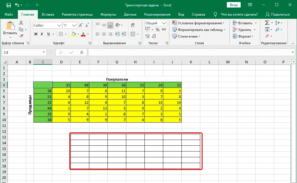
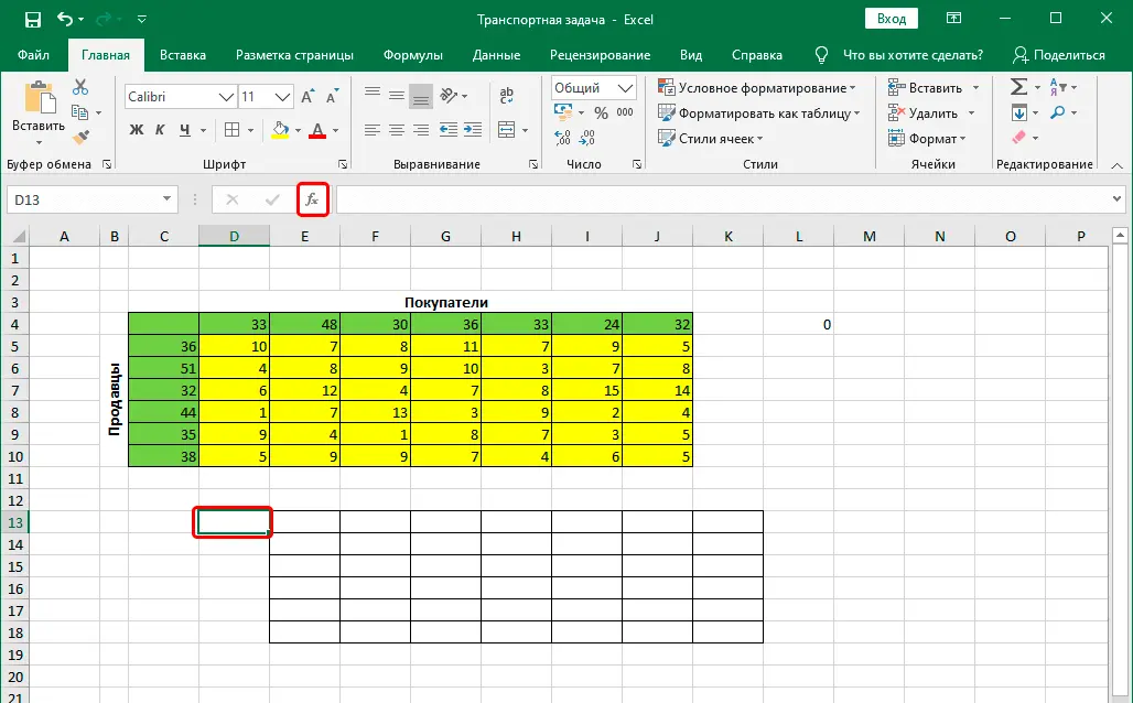
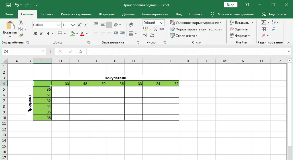
Suppose we have 6 sellers and 7 buyers. Demand and supply between them are distributed respectively in the following way: 36, 51, 32, 44, 35 and 38 units are sellers and 33, 48, 30, 36, 33, 24 and 32 units are buyers. If you sum up all these values, you will find that supply and demand are in balance. Therefore, this problem is of a closed type, which is solved very simply.
In addition, we have information about how much you need to spend on transportation from point A to point B (they are highlighted in yellow cells in the example). 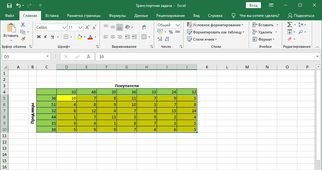
Solution – step by step algorithm
Now, after we have familiarized ourselves with the tables with the initial data, we can use the following algorithm to solve this problem:
- First, we make a table consisting of 6 rows and 7 columns.

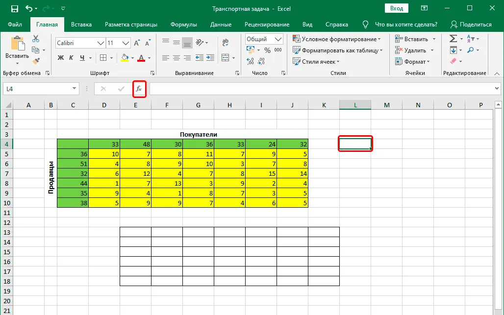
- After that, we go to any cell that does not contain any values and at the same time lies outside the newly created table and insert the function. To do this, click on the fx button, which is located to the left of the function entry line.

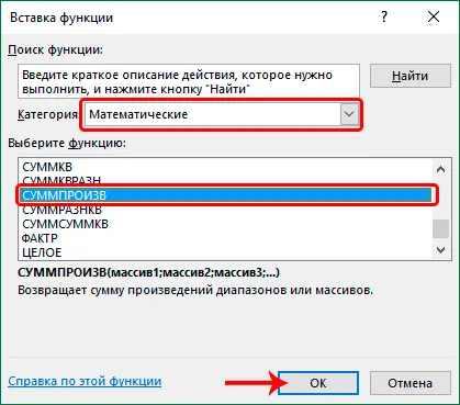
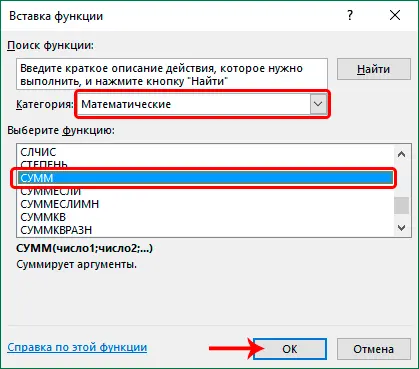
- We have a window in which we need to select the category “Math”. What function are we interested in? The one highlighted in this screenshot. Function SUMPRODUCT multiplies ranges or arrays among themselves and sums them. Just what we need. After that, press the OK key.

- Next, a window will appear on the screen in which you need to specify the function parameters. They are the following:
- Array 1. This is the first argument in which we write the range that is highlighted in yellow. You can set the function parameters either using the keyboard or by selecting the appropriate area with the left mouse button.
- Array 2. This is the second argument, which is the newly created table. Actions are performed in the same way.
Confirm your action by pressing the OK button. 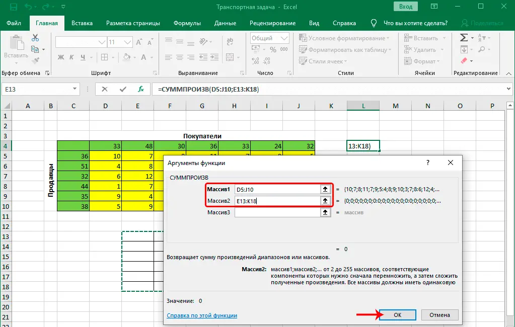
- After that, we make a left mouse click on the cell that serves as the top left in the newly created table. Now click the insert function button again.

- We select the same category as in the previous case. But this time we are interested in the function SUM.

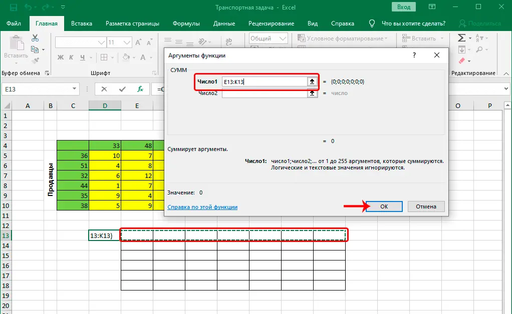
- Now comes the stage of filling in the arguments. As the first argument, we write the top row of the table that we created at the beginning. In the same way as before, this can be done by selecting these cells on the sheet, or manually. We confirm our actions by pressing the OK button.

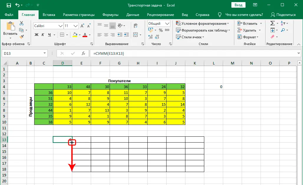
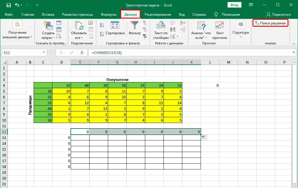
- We will see the results in the cell with the function. In this case, it’s zero. Next, move the cursor to the lower right corner, after which an autocomplete marker will appear. It looks like a little black plush. If it appears, hold down the left mouse button and move the cursor to the last cell in our table.

- This gives us the opportunity to transfer the formula to all other cells and get the correct results without having to perform additional calculations.
- The next step is to select the top left cell and paste the function SUM into her. After that, we enter the arguments and use the autocomplete marker to fill in all the remaining cells.
- After that, we proceed directly to solving the problem. To do this, we will use the add-on that we included earlier. Go to the “Data” tab, and there we find the “Search for a solution” tool. We click on this button.

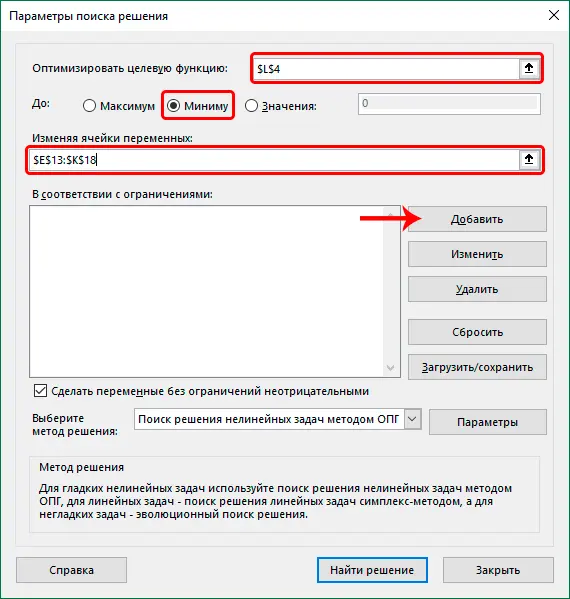
- Now a window has appeared before our eyes, through which you can configure the parameters of our add-on. Let’s take a look at each of these options:
- Optimize the objective function. Here we need to select the cell containing the function SUMPRODUCT. We see that this option makes it possible to select a function for which a solution will be searched.
- Before. Here we set the option “Minimum”.
- By changing the cells of the variables. Here we indicate the range corresponding to the table that we created at the very beginning (with the exception of the summarizing row and column).
- Subject to restrictions. Here we need to add constraints by clicking the Add button.

- We remember what kind of constraint we need to create – the sum of the values of buyers’ demands and sellers’ offers must be the same.
- The task of restrictions is carried out as follows:
- Link to cells. Here we enter the range of the table for calculations.
- Terms. This is a mathematical operation against which the range specified in the first input field is checked.
- The value of the condition or constraint. Here we enter the appropriate column in the source table.
- After all the steps are completed, click the OK button, thereby confirming our actions.
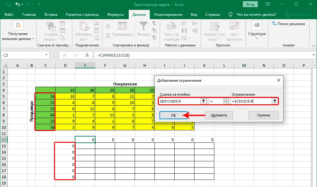
We perform exactly the same operations for the top rows, setting the following condition: they must be equal. 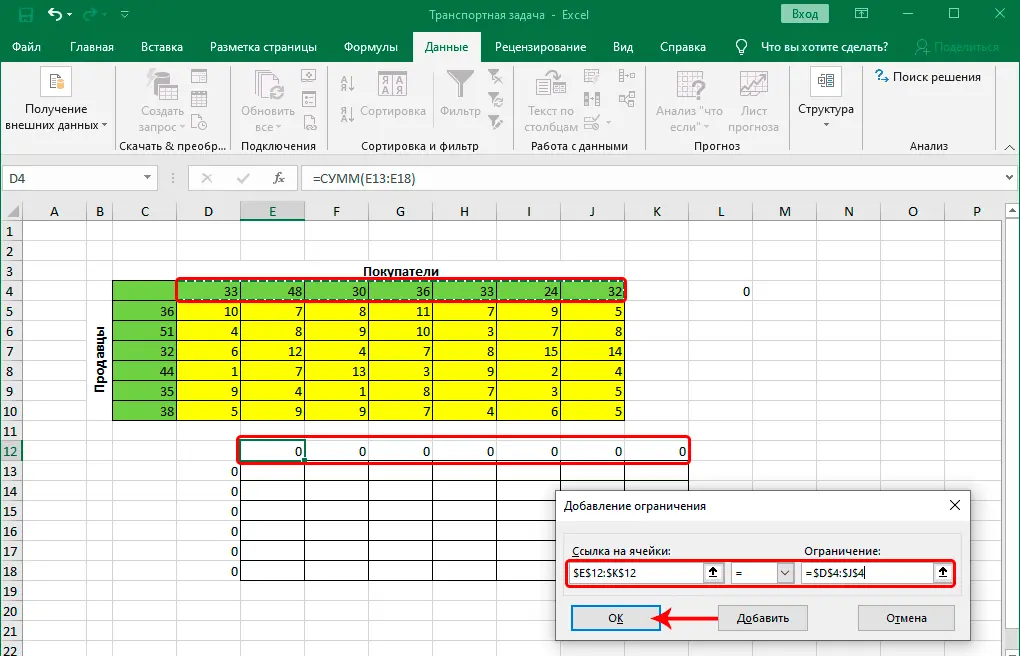
The next step is setting the conditions. We need to set the following criteria for the sum of the cells in the table – greater than or equal to zero, an integer. As a result, we have such a list of conditions under which the problem is solved. Here you need to make sure that the checkbox next to the option “Make variables without limits non-negative” is checked. Also, in our situation, it is required that the method for solving the problem is chosen – “Searching for a solution to nonlinear problems of OPG methods”. Now we can safely say that the setting is done. Therefore, it remains only to perform the calculations. To do this, click on the “Find a solution” button. 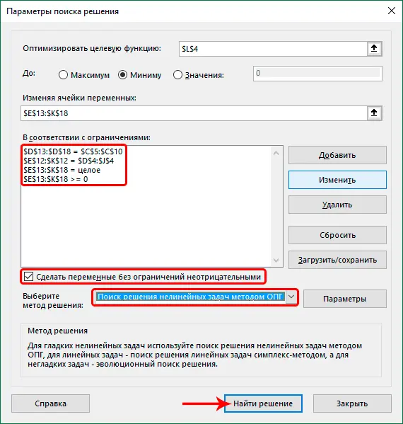
After that, all data will be calculated automatically, and then Excel will show a window with the results. It is necessary in order to double-check the operation of the computer, since errors are possible if the conditions were previously set incorrectly. If everything is correct, then click the “OK” button and see the finished table.
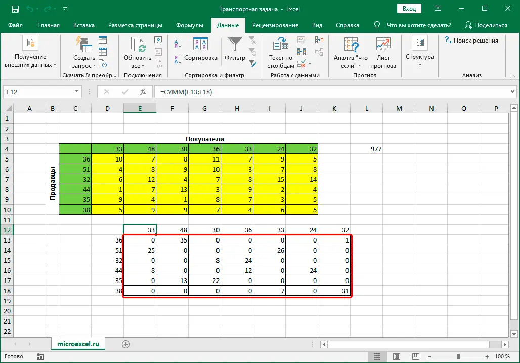
If it turns out that our task has become an open type, then this is bad, because you need to edit the source table so that the task turns into a closed one. However, when this is done, the remaining algorithm will be the same.
Conclusion
As you can see, Excel can also be used for very complex calculations, which at first glance are not available to a simple computer program that is installed in almost everyone. However, it is. Today we have already covered the advanced level of use. This topic is not so simple, but as they say, the road will be mastered by the walking one. The main thing is to follow the action plan, and accurately perform all the actions indicated above. Then there will be no errors, and the program will independently perform all the necessary calculations. There will be no need to think about which function to use and so on.


