


Excel users very often have to deal with the need to calculate the average value. There are several methods for obtaining an average, each with its own advantages and disadvantages. But the most common is to obtain the arithmetic mean. To get it, you need to add all the numbers in the row together, and then divide them all by their total number.
That is, the formula itself is not very complicated. And if you do it in Excel, everything will be even easier. Let’s take a closer look at what needs to be done to achieve this goal.
About the status bar in Excel
If we only need to know the average value, there is no need to get it using formulas. You can see it in the status bar. This is the most convenient method, which, among other things, is the easiest to implement. 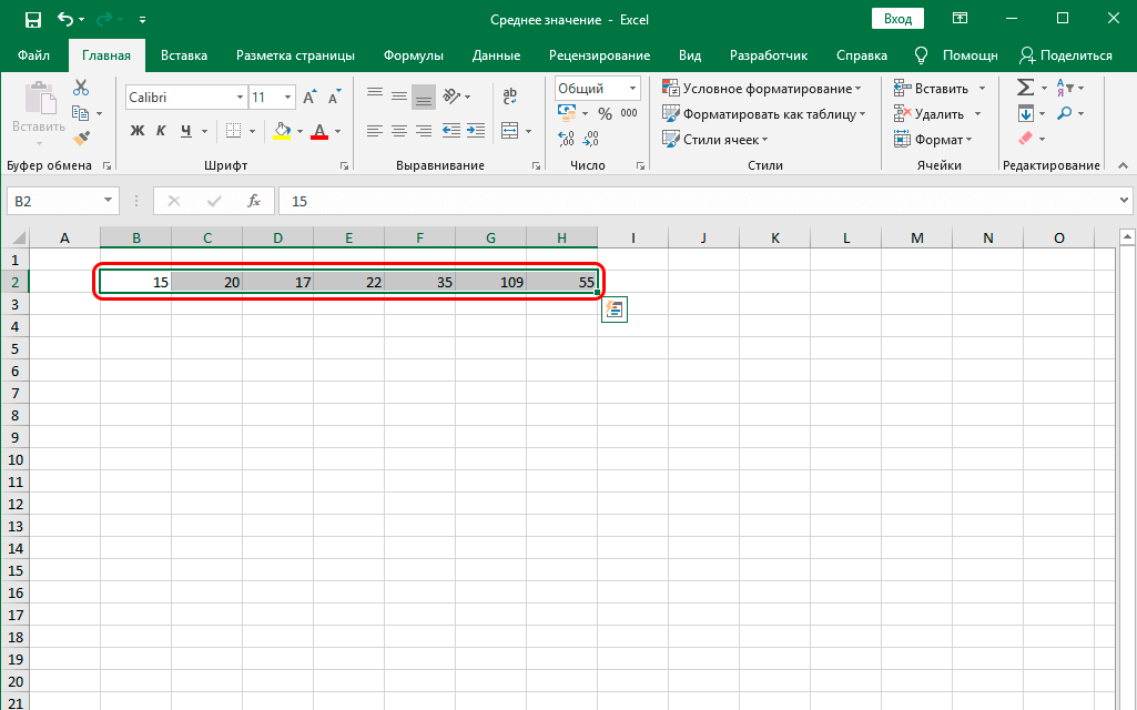
If you cannot read this information, then this may be due to the fact that this option is disabled in the settings. To activate it, you need to right-click on the status bar and find the inscription “Average” in the list. Then click on this item with the left button once.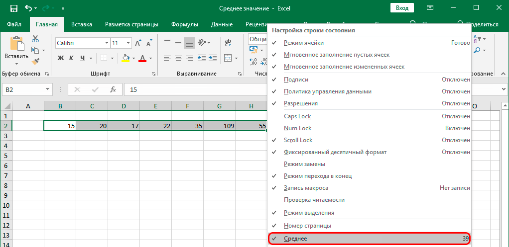
6 Ways to Calculate Average in Excel
Now let’s move on to more professional methods for getting the arithmetic mean. They are necessary in cases where it is necessary not only to calculate it, but also to write it in a specific cell. Further, its contents will be used for calculations or simply for visual acquaintance with information that is constantly updated. After all, all the methods described above allow you not to revise the average value every time the contents of the cells with the data underlying it change.
How to determine the average value by condition
One of the most interesting features that allows you to determine the average value is the ability to calculate it based on a pre-specified condition. That is, the program will take into account only the values corresponding to a specific criterion. For example, we should take the arithmetic mean of only those numerical values that are greater than zero. In this situation, you need a function HEARTLESS. To use it, you need to perform the following sequence of steps:
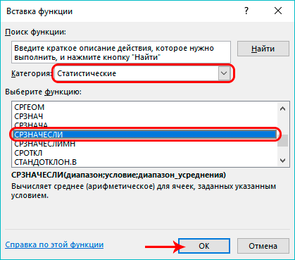
- Determine the cell involved in the calculations. Left click on it once. Find the fx button to the left of the formula input line, which will open the function insertion dialog box.

- In the window that appears, find the statistical functions and find the operator in the list HEARTLESS. To select it, you must first open the list with categories, find the one described above and click on it. A list of functions will appear, in which you also need to left-click on the function. Then you can confirm your actions by pressing the enter key or the OK button with the mouse.
- A list of function arguments will appear. These are the values that we pass to it, as well as the parameters used for calculations. The function provides the following arguments:
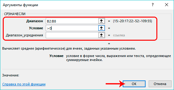
- Range. This is the area of cells that is taken into account by the function. You can specify it both manually and by selecting the appropriate cells and / or ranges in the sheet itself.
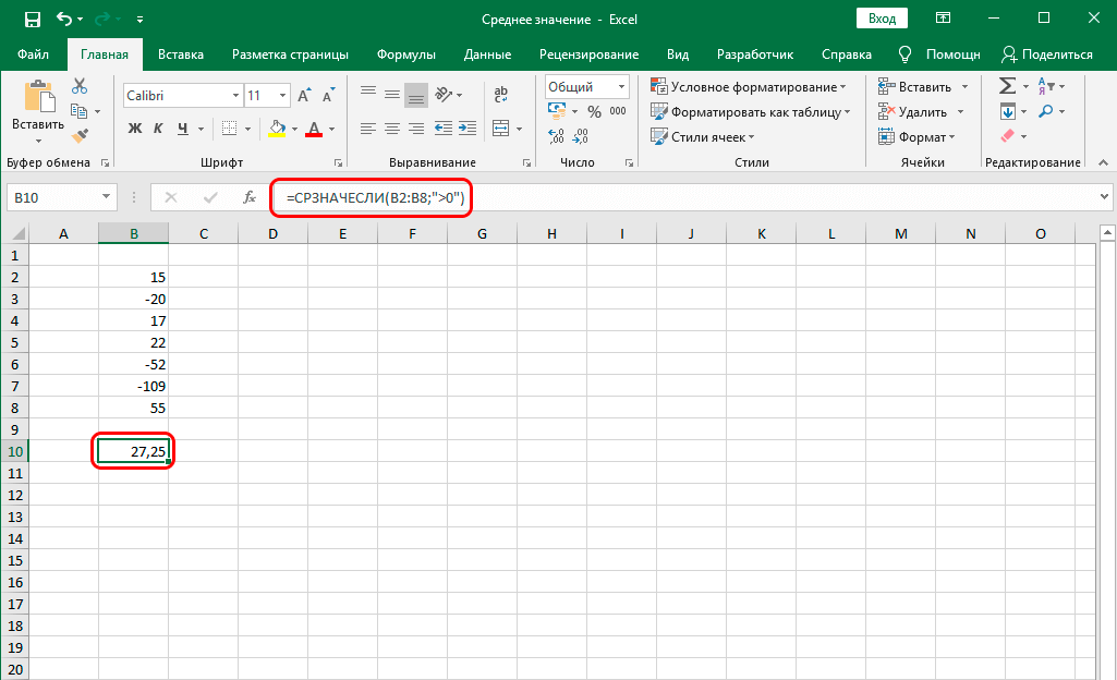
- Condition. Here you set the criterion that will be taken into account when selecting values for averaging. Since we need to sum up all cells that contain a positive number, the condition must be written as follows: > 0. That is, the comparison operator is used first, and then the number itself is written.
- Averaging range. This field can be left blank as it is not needed in a table that does not contain text values.
- Next, we confirm our actions, and the average value will appear in the desired cell.
Entering a function into a cell manually
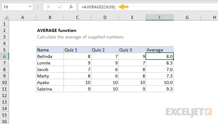
And now it’s time to get acquainted with the main function of calculating the average – AVERAGE. We will talk a lot more about her. It has this syntax: =CORE(number1;2;3). As you can see, the syntax of this function is very simple. You need to write the operator itself, and then, separated by a semicolon, list the numbers, cells or ranges that are taken into account for calculating the arithmetic mean.
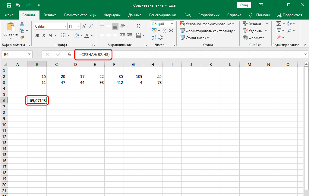
To write a function AVERAGE with your own hands, you need to write the = sign in the cell (this is the universal symbol for entering the formula), and then write in capital letters AVERAGE (the program will automatically prompt this function in the list, so it will be enough to click on the prompt with the left mouse button once), then open the bracket and enter the arguments. Arguments can be entered in several ways. The easiest is to click on the corresponding cells or highlight the corresponding ranges. After that, you need to put a separator – a semicolon (;) and enter the next value. You can also just write a number as an argument. The bracket is then closed and the enter key is pressed. Then the arithmetic mean of the values will automatically appear in the desired cell. For example, this is how a formula looks like that finds the arithmetic mean of numbers in a table that is on the second and third rows.
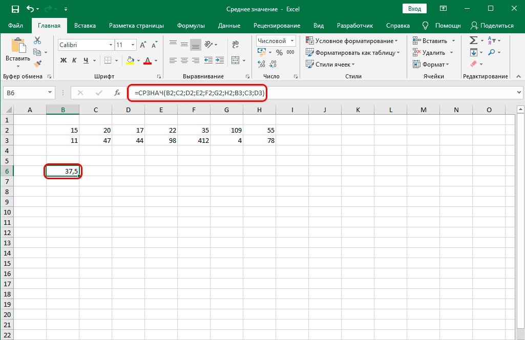
We see that the arithmetic mean of all these values is 37,5. For many people, this method will not seem convenient. However, if you master the blind typing method, then entering any data from the keyboard will be much faster than manually selecting all the necessary data. In addition, it will be much easier to use the manual method of finding the arithmetic mean for those people who already know this function by heart. If the user is just learning to use Excel, then other methods will suit him.
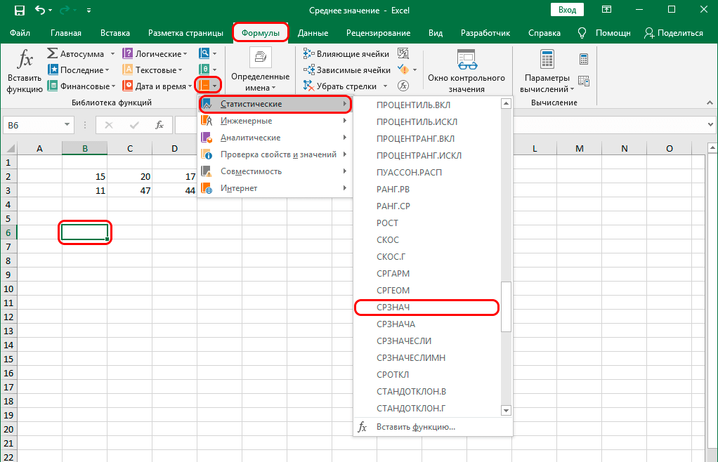
Determining the average value using the tools in the “Formulas” tab
If a person does not use spreadsheets very easily or he does not want to enter too much data from the keyboard, then Excel provides a tab that allows you to insert formulas. In particular, it can be used to obtain the arithmetic mean of a numerical range or a set of cells. What should be done?
- Click on the cell where the arithmetic mean will be calculated.
- We find the “Formulas” tab in the menu. Next, go to the “Library of Functions” section. By default, it is not displayed with a caption, but for clarity, we will demonstrate where this button is located.
- After we click on this button, a list of functions will appear. We are interested in the “Statistical” section, and then – AVERAGE.
- Next, a window for entering function arguments will appear. Here you can set your own numbers, select cells to include in the range, or select the range of values directly. We’ll take the final step.

Calculation of the average value using the AVERAGE formula
As we already understood, the basic formula for calculating the arithmetic mean is AVERAGE. You can either enter it manually or select it directly in the formula input field. Let’s now master this feature at an advanced level.
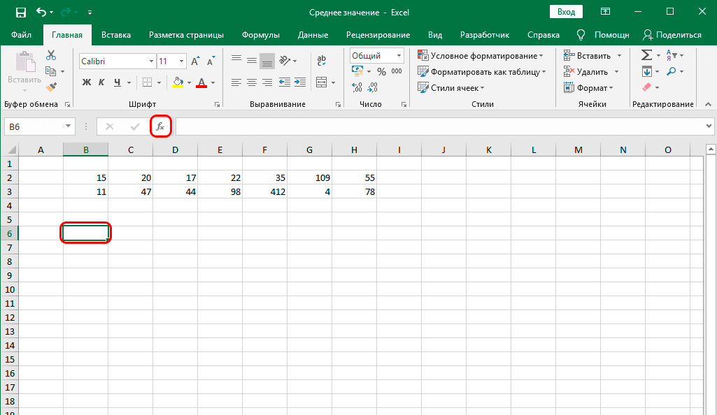
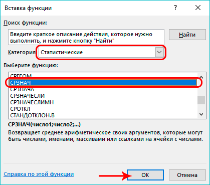
- Select the cell in which the program should write the result. To do this, click on the insert function button, which we already know.
- The window that opens is called the Function Wizard. Here you need to select the category and the name of the function. Only this time we are interested in the function AVERAGEAnd not HEARTLESS. After we make a left mouse click on it, click OK.
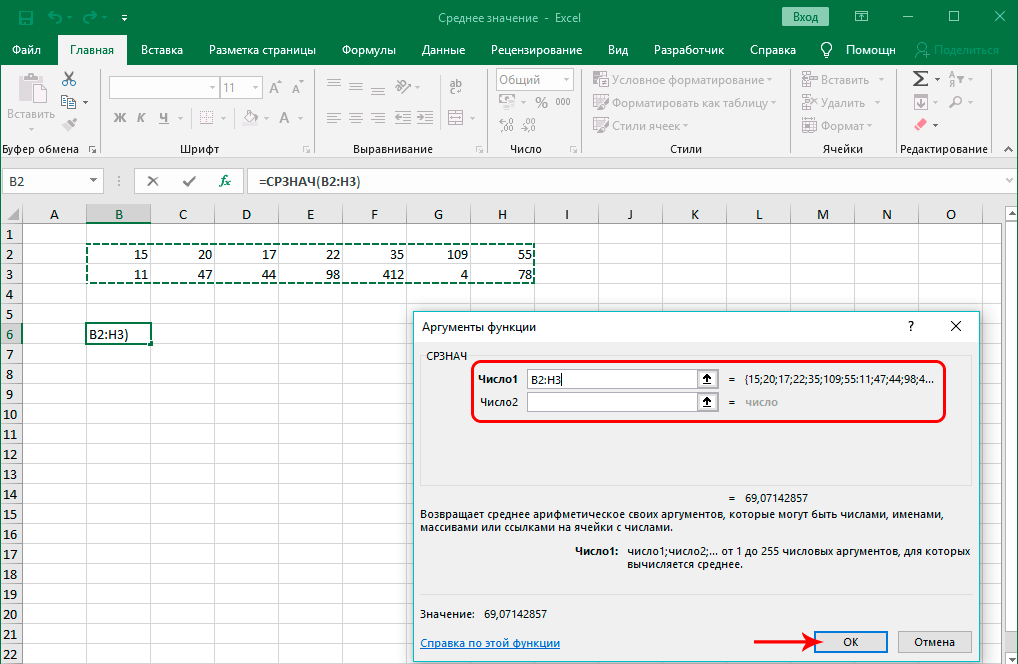
- Then a dialog box with function settings will appear. The maximum number of arguments that can be used is 255. But the number of numbers itself is much larger. Just the maximum you can use is 255 ranges, but they can be of different sizes. Entering arguments can be either in manual mode or by selecting the appropriate cells with the mouse. If you need to insert a range, then you just need to select them in the same way as any other values. If necessary, you can select a range that is located elsewhere in the table as the second, third, and so on arguments. You can confirm your actions with the OK key.
- The result will be in the cell that was selected in the first step.
Very often there is a situation where the average value does not look very good. The reason for this is the large number of decimal places. If there is no need to transmit data so accurately, then it is better to remove unnecessary numbers. To do this, the context menu is called (right-click on the corresponding cell), and then click on the “Format Cells” item. 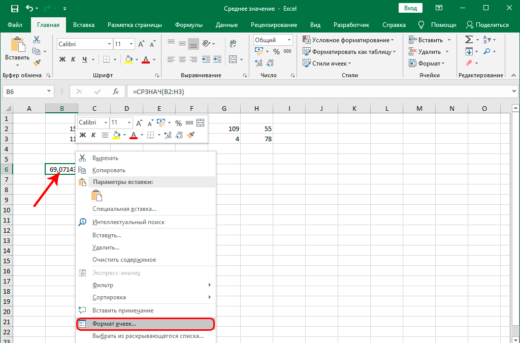
The first tab that will be selected by default is Number. If suddenly another one was opened, then you need to go to it. On the left side of the window there is a list of format types, we need to select “Numeric”. On the right side of the window there is an item “Number of decimal places”, and even to the right there is a switch in which you can set the number of decimal places. The user can also set a separator for groups of digits by checking the corresponding box. 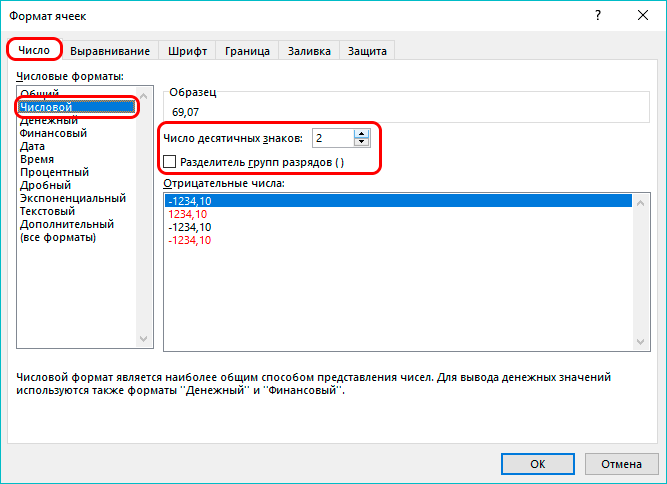
After we confirm our actions, the cell that was selected in the first step will display the average value of the range that we selected, with as many decimal places as we need.
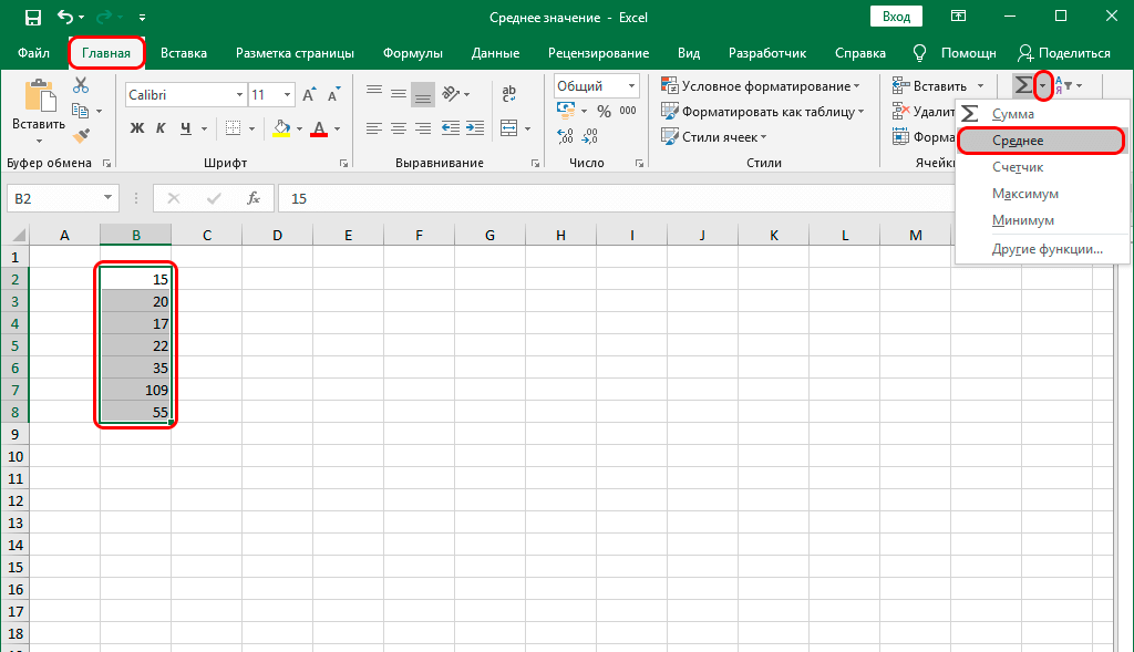
Ribbon Tools for Mean Calculation
The main menu in Excel is called the ribbon. It has special tools that allow you to calculate the average value. First, we need to select the range that will serve as the basis for determining the average value.
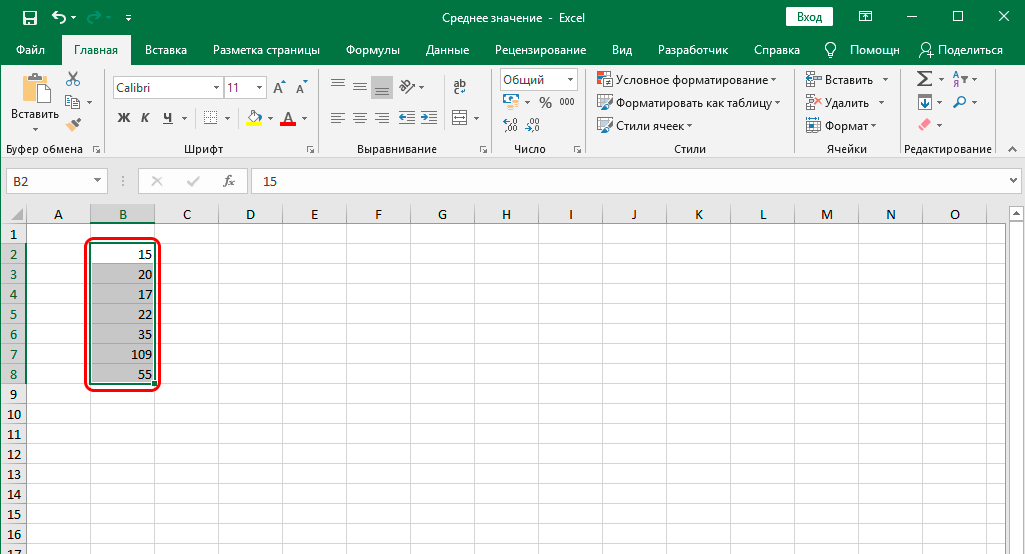
Then we go to the “Home” tab, if another section was open at that moment. Next, we find the “Editing” subsection, in which we are looking for the “Autosum” icon. But we do not click on this icon, but on the arrow, which is located slightly to the right of it. After that, an additional menu will open, in which you can select different formulas in order to carry out a quick calculation. We find the item “Average” there and click on it.
Next, we will see the result, just below the range that was selected. This method can save you a lot of time if you want to get the result directly in the cell below the range. It is enough to make just a couple of clicks, and the result is in your pocket.
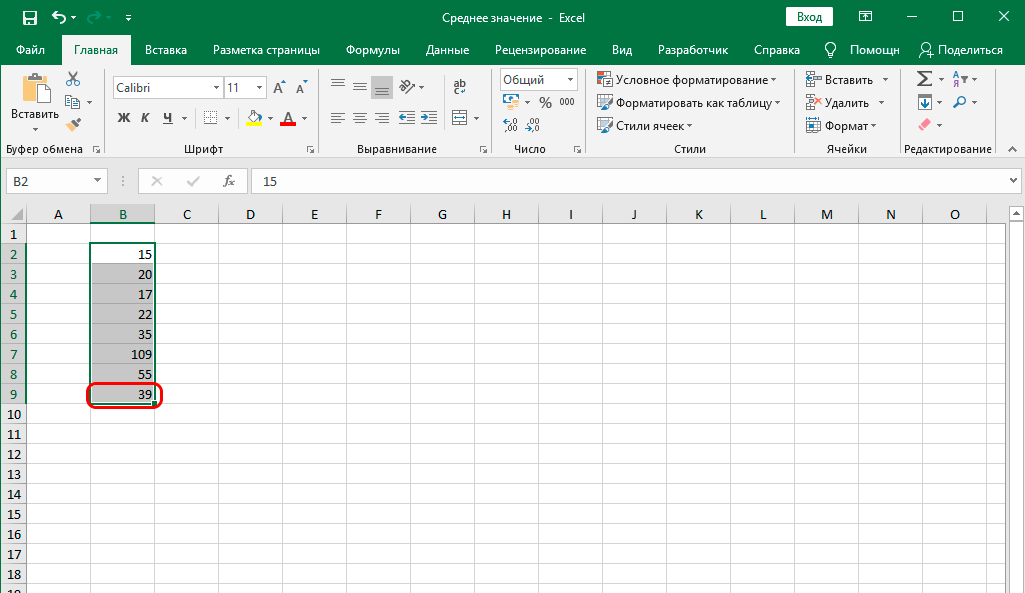
If we click on this cell, we will see the familiar function in the formula bar AVERAGE.
The tool can also be used to find the average of a range that is horizontal instead of vertical. In this case, the final result will be displayed to the right of it.
Using an arithmetic expression
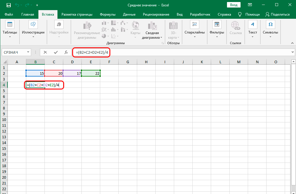
You can also use the standard mathematical formula if the number of values for which you want to find the arithmetic mean is small. To do this, you need to perform the following sequence of actions:
- Click on the cell in which the final result will be displayed. After that, we write the formula input sign (=) and write the following formula: =(Number1+Number2+Number3…)/Number_of_terms. In brackets, you can specify not only a number, but also give a direct link to the cell. For example, let’s define the arithmetic mean of the numbers contained in cells B2, C2, D2 and E2. How the formula will look in the end can be seen in this screenshot if you look at the formula bar.
- After the formula is entered, we confirm our actions by pressing the enter key.
This is the most obvious method that can be used to determine the arithmetic mean. But it is very poorly suited if you need to process large amounts of information. After all, it can take a huge amount of time to list all the cells or numeric values. Yes, it is easy to make a mistake when entering manually. In general, the user can choose the method that he likes. If there is little data, you can manually enter it, the loss of time will not be significant. And if there is a lot of data, then it is better to use other tools, of which there are a huge number.