


Video
Formulation of the problem
We have a table with which we constantly have to work (sort, filter, count something on it) and the contents of which periodically change (add, delete, edit). Well, at least, for an example – here it is like this:
The size – from several tens to several hundred thousand lines – is not important. The task is to simplify and make your life easier in every possible way by turning these cells into a “smart” table.
Solution
Select any cell in the table and on the tab Home (Home) expand the list Format as a table (Format as table):
In the drop-down list of styles, select any fill option to our taste and color, and in the confirmation window for the selected range, click OK and we get the following output:
As a result, after such a transformation of the range into “smart” Table (with a capital letter!) we have the following joys (except for a nice design):
- Created Table gets a name Table 1,2,3 etc. which can be changed to a more adequate one on the tab Constructor (Design). This name can be used in any formulas, drop-down lists, and functions, such as a data source for a pivot table or a lookup array for a VLOOKUP function.
- Created once Table automatically adjusts to size when adding or deleting data to it. If you add to such Table new lines – it will stretch lower, if you add new columns – it will expand in breadth. In the lower right corner Tables you can see the automatically moving border marker and, if necessary, adjust its position with the mouse:
- In the hat Tables automatically AutoFilter turns on (can be forced to disable on the tab Data (Date)).
- When adding new lines to them automatically all formulas are copied.
- When creating a new column with a formula – it will be automatically copied to the entire column – no need to drag formula with black autocomplete cross.
- When scrolling Tables down column headings (A, B, C…) are changed to field names, i.e. you can no longer fix the range header as before (in Excel 2010 there is also an autofilter):
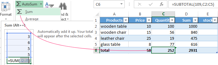
- By enabling the checkbox Show total line (Total row) tab Constructor (Design) we get an automatic totals row at the end Tables with the ability to select a function (sum, average, count, etc.) for each column:
- To the data in Table can be addressed using the names of its individual elements. For example, to sum all the numbers in the VAT column, you can use the formula =SUM(Table1[VAT]) instead =SUM(F2:F200) and not to think about the size of the table, the number of rows and the correctness of the selection ranges. It is also possible to use the following statements (assuming the table has the standard name Table 1):
- =Table1[#All] – link to the entire table, including column headers, data and total row
- =Table1[#Data] – data-only link (no title bar)
- =Table1[#Headers] – link only to the first row of the table with column headings
- =Table1[#Totals] – link to the total row (if it is included)
- =Table1[#This row] — reference to the current row, for example, the formula =Table1[[#This row];[VAT]] will refer to the VAT value from the current table row.
(In the English version, these operators will sound, respectively, as #All, #Data, #Headers, #Totals and #This row).
PS
In Excel 2003 there was something remotely similar to such “smart” tables – it was called the List and was created through the menu Data – List – Create List (Data — List — Create list). But even half of the current functionality was not there at all. Older versions of Excel didn’t have that either.