How to Convert Rows to Columns in Excel

This guide explains what to do to convert rows to columns in Excel. When using Excel, you often have to swap rows and columns in a table. For example, it happens that a person has made a huge table, and then he realized that it is much easier to read it if you turn it over. 

Эта детальная инструкция расскажет о нескольких способах транспонирования Excel-таблицы, а также о часто встречаемых ошибках, с которыми может столкнуться пользователь. Все они могут использоваться на любой версии Excel, как очень старой, так и самой новой.

Using the Paste Special feature

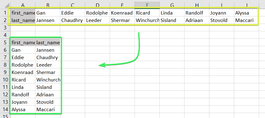
Let’s say you have two datasets. The second is what you want to end up with. The first is the table that needs to be transposed. In the first version, the names of countries are presented in different columns, and it is very inconvenient to read, and even more so, to compare the characteristics of states with each other. Therefore, it is much better to organize the table so that the country names appear in different columns.

To swap rows and columns, do the following:

1. Select the original table. If you want to see the whole table at once (if it is very large), you need to press the key combination Ctrl + Home, and after that – Ctrl + Shift + End.
2. The cells are then copied. This can be done either through the context menu or by pressing the Ctrl+C key combination. It is recommended that you immediately accustom yourself to the last option, because if you learn hot keys, you can perform many tasks literally in one second.
3. Select the first cell in the target range. При этом он должен находиться за пределами таблицы. Также необходимо подобрать ячейку таким образом, чтобы таблица после транспонирования не пересекалась с другими данными. For example, if the initial table has 4 columns and 10 rows, then after performing all these operations, it will spread 10 cells down and 4 cells to the side. Therefore, within this range (counting from the target cell) there should be nothing.
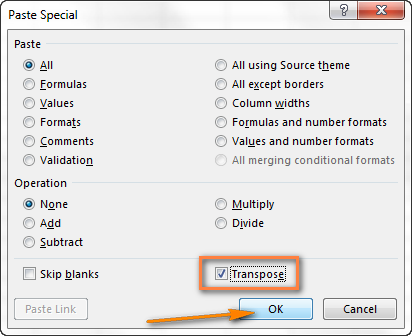
4. On the target cell, you must right-click and select “Paste Special”, and then check the box next to the inscription “Transpose”.

Important: if there are formulas in the source table, it is important to ensure that absolute references are used in each cell. This must be done so that all links are automatically updated.

Огромное преимущество опции «Специальная вставка» и заключается в возможности транспонировать таблицу всего лишь за несколько секунд. И при этом полностью сохраняется форматирование, что также позволяет сэкономить кучу времени.

Несмотря на эти явные плюсы, есть и ряд серьезных недостатков, которые мешают этому методу называться универсальным:

1. It is bad to use it for transposing full-fledged tables that are not reduced to a banal range of values. In this case, the “Transpose” function will be disabled. To work around this issue, you must convert the table to a range.
2. This method is well suited for a one-time transpose because it does not associate the new table with the original data. In simple words, when you change one of the tables, the information will not be automatically updated on the second. Therefore, the transposition will have to be repeated. 

How to swap rows and columns and link them to the main table?

So, what can be done so that the “Paste Special” option can link the table with the main data and the one resulting from the transposition? After all, everyone would like the data to be automatically updated.

1. Скопировать таблицу, для которой требуется транспонирование.
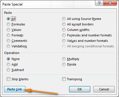
2. Select a cell with no data in an empty area of ​​the table.
3. Launch the Paste Special menu, similar to the previous example. After that, you need to click on the “Insert link” button, which can be found at the bottom left.
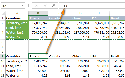
4. The result will be the following.
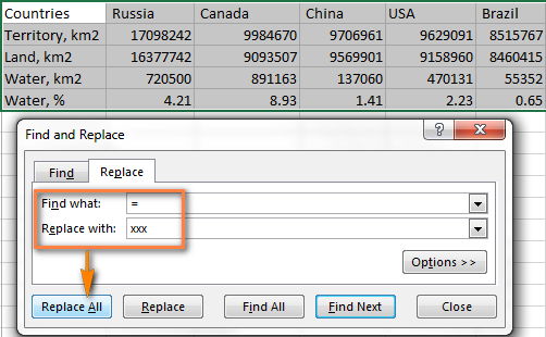
5. Выбрать новую таблицу и запустить окно «Найти и заменить» путем нажатия комбинации клавиш Ctrl + H.
6. Заменить все знаки ввода формулы (=) на ххх (или любую другую комбинацию знаков, которой нет в оригинальной таблице).
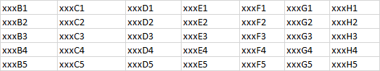
7. As a result, something terrible will turn out, but this is an obligatory intermediate condition for achieving the desired result. Then everything will look beautiful.
8. Copy the resulting table and then use Paste Special to transpose it.

After that, you just need to re-open the “Find and Replace” dialog, and use it to change the “xxx” in the cells to “=” so that all cells are associated with the original information.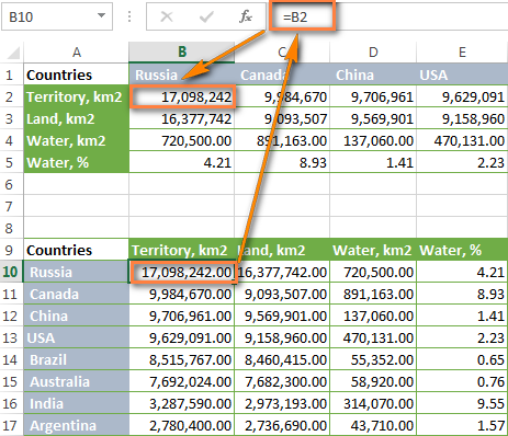Of course, this is more complicated and longer, but this method allows you to get around the lack of a link to the original table. But this approach also has a drawback. It is expressed in the need to independently resume formatting.

Application of formulas

There are two functions that allow you to flexibly change rows and columns: ТРАНСП и ДВССЫЛ. Здесь также есть возможность сохранить связь с первоначальной таблицей, но механика работы несколько иная.

function TRANSP

Actually, this formula directly transposes the spreadsheet. The syntax is the following:

=TRANSP(array)

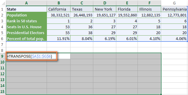
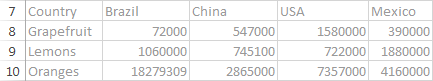
Now we will try to apply it to a table that contains information about the population of individual states.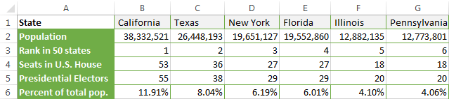

1. Count the number of columns and rows in the table and find an empty space in the sheet that has the same dimensions.
2. Start edit mode by pressing the F2 key.
3. Write a function TRANSP with the data range in brackets. It is important to always use absolute references when using this function.
4. Press the key combination Ctrl+Shift+Enter. It is important to press exactly the key combination, otherwise the formula will refuse to work.

That’s it, now the result looks like this!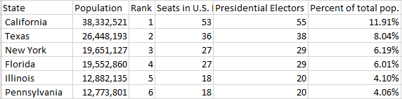

The advantage of this formula is the same as the previous method (using the “find and replace” function) is that when the underlying information changes, the transposed table will automatically update.

Но недостатки у нее тоже имеются:

1. Formatting, as in the case of the Find and Replace method, will not be saved.
2. The original table must contain some data, otherwise there will be zeros in some cells.
3. Излишняя зависимость от источника данных. То есть, этот метод имеет противоположный по недостаток – невозможность изменять транспонированную таблицу. Если попытаться это сделать, программа скажет, что невозможно редактировать часть массива.

Also, this function can not always be applied flexibly in different situations, so you need to know about it, but use more efficient techniques.

Using the INDIRECT Formula

The mechanics of this method is very similar to using the formula TRANSP, но при этом его использование решает проблему невозможности редактировать транспонированную таблицу без потери связи с основной информацией.

Но одной формулы INDIRECT not enough: you still need to use the function ADDRESS. There will be no large table in this example, so as not to overload you with a lot of unnecessary information.

So, let’s say you have such a table, consisting of 4 columns and 5 rows.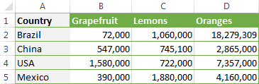

The following actions need to be taken:

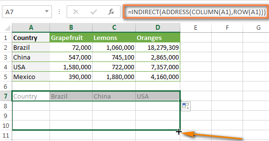
1. Enter this formula: =INDIRECT(ADDRESS(COLUMN(A1),ROW(A1))) into the upper left cell of the new table (in our example it is A7) and press the enter key. If the information does not start in the first row or the first column, then you will have to use a more complex formula: =ДВССЫЛ(АДРЕС(СТОЛБЕЦ(A1)-СТОЛБЕЦ($A$1)+СТРОКА($A$1);СТРОКА(A1)-СТРОКА($A$1)+СТОЛБЕЦ($A$1))). In this formula, A1 means the top cell of the table, on the basis of which the transposed cell will be formed.
2. Extend the formula to the entire area where the new version of the table will be placed. To do this, drag the marker in the lower right corner of the first cell to the opposite end of the future table.
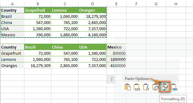
3. All! The table turned out to be successfully transposed, and you can still edit it. Of course, her appearance leaves much to be desired, but fixing it is not difficult. To restore the correct formatting, you need to copy the table that we transposed (that is, the original one), then select the newly created table. Next, right-click on the selected range, and then click on “Formatting” in the paste options.

So using the function INDIRECT allows you to edit absolutely any value in the final table, and the data will always be updated as soon as any changes are made in the source table.

Of course, this method is more difficult, but if you work it out in practice, then everything is not so scary.

Этот метод один из самых лучших, потому что несмотря на то, что не сохраняется форматирование в новосозданной таблице, можно его легко восстановить.

How does the combination of INDIRECT and ADDRESS formulas work?

После того, как вы разобрались в том, как использовать совокупность этих формул для транспонирования таблицы, вам, возможно, захочется более глубоко изучить принцип работы этого метода.

Function INDIRECT in our formula is used to create an indirect cell reference. For example, if you need to specify the same value in cell A8 as in B1, then you can write the formula

=INDIRECT(“B1”)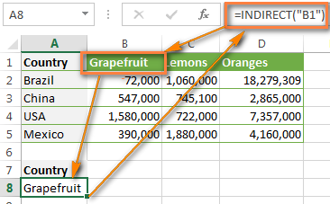

Казалось бы, зачем это делать? Ведь можно просто написать ссылку на ячейку в другой ячейке. Но преимущество этой функции в том, что в ссылку можно превратить абсолютно любую строку, и даже ту, которая создается с использованием других формул. Собственно, это мы и делаем в формуле.

Beyond Function ADDRESS also used in the formula COLUMN и LINE. The first returns the address of the cell based on the already known row and column numbers. It is important to follow the correct sequence here. First the row is specified, and then only the column. For example, the function ADDRESS(4;2) will return the address $B$2.

Следующая используемая выше функция – это COLUMN. It is necessary here so that the formula receives the column number from a specific reference. For example, if you use the B2 parameter in the brackets of this function, then it will return the number 2, since the second column is column B.

Obviously, the ROW function works the same way, it just returns the row number. 

And now we will use not abstract examples, but a very specific formula that was used above:

=INDIRECT(ADDRESS(COLUMN(A1),ROW(A1)))

Here you can see that first in the function ADDRESS the column is specified, and only then the line. And it is here that the secret of the working capacity of this formula is hidden. We remember that this function works in a mirror way, and the first argument in it is the line number. And it turns out that when we write the address of a column there, it turns into a line number and vice versa.

То есть, если подытожить:

1. We get the column and row numbers using the corresponding functions.
2. Using the function ADDRESS rows become columns and vice versa.
3. Function INDIRECT helps to display the mirrored data in the cell.

That’s how simple it all turns out!

Using a macro to transpose

A macro is a small program. It can be used to automate the process. It is important to consider that the macro has some limitations. The maximum Transpose method allows you to work with 65536 elements. If this limit is exceeded, it will result in data loss.

Во всем остальном, это эффективный метод автоматизации, который сможет значительно облегчить жизнь.

Например, можно написать такой код, который будет менять местами строки и колонки.

Sub TransposeColumnsRows()

    Dim SourceRange As Range

    Dim DestRange As Range

    Set SourceRange = Application.InputBox(Prompt:=»Please select the range to transpose», Title:=»Transpose Rows to Columns», Type:=8)

    Set DestRange = Application.InputBox(Prompt:=»Select the upper left cell of the destination range», Title:=»Transpose Rows to Columns», Type:=8)

    SourceRange.Copy

    DestRange.Select

    Selection.PasteSpecial Paste:=xlPasteAll, Operation:=xlNone, SkipBlanks:=False, Transpose:=True

    Application.CutCopyMode = False

End Sub

Но если знаний в программировании особо нет, ничего страшного. Можно воспользоваться описанными выше способами. А потом учиться новому по мере освоения старого.