


Contents
Visual presentation of information helps to facilitate its perception. Probably the easiest way to turn dry data into a visually accessible form is to create graphs and tables. No analyst can do without them.
Graphs have a number of advantages over other ways of visually presenting information. First, they allow you to quickly process the available numerical values and make certain predictions. Among other things, planning allows you to check the validity of the available numerical data, since inaccuracies may appear after the creation of the schedule.
Thank God Excel makes creating charts a simple and easy process, just based on existing numerical values.
Creating a graph in Excel is possible in different ways, each of which has significant advantages and limitations. But let’s look at everything in more detail.
Elementary change graph
A graph is needed if a person is required to demonstrate how much a certain indicator has changed over a specific period of time. And the usual graph is quite enough to complete this task, but various elaborate diagrams can actually only make the information less readable.
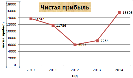
Suppose we have a table that provides information about a company’s net income over the past five years.
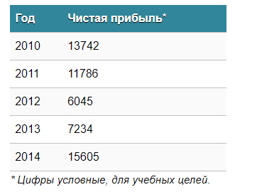
Important. These figures do not represent actual data and may not be realistic. They are provided for educational purposes only.
Then go to the “Insert” tab, where you have the opportunity to select the type of chart that will be suitable for a particular situation.
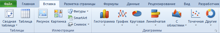
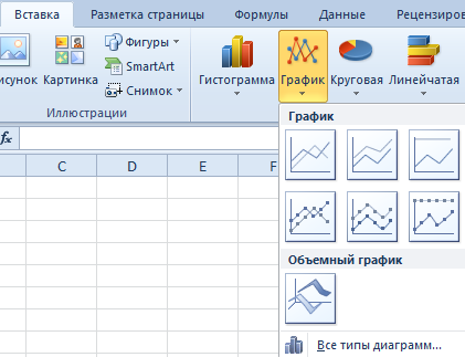
We are interested in the “Graph” type. After clicking on the corresponding button, a window with settings for the appearance of the future chart will appear. To understand which option is appropriate in a particular case, you can hover your mouse over a specific type and a corresponding prompt will appear.
After selecting the desired type of chart, you need to copy the data table and link it to the graph. The result will be the following.
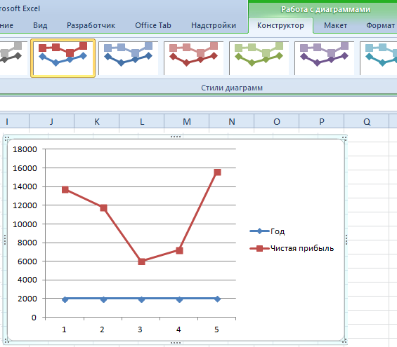
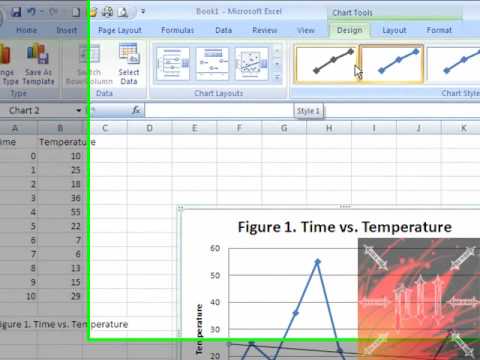
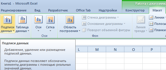
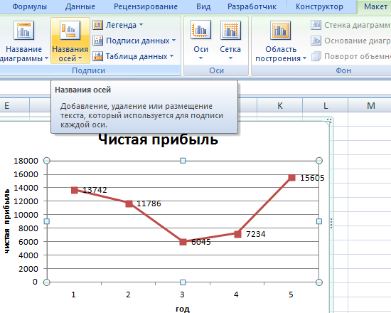
In our case, the diagram shows two lines. The first one is red. The second is blue. We do not need the latter, so we can remove it by selecting it and clicking the “Delete” button. Since we have only one line, the legend (a block with the names of individual chart lines) can also be removed. But markers are better named. Find the Chart Tools panel and the Data Labels block on the Layout tab. Here you have to determine the position of the numbers.
The axes are recommended to be named to provide greater readability of the graph. On the Layout tab, find the Axis Titles menu and set a name for the vertical or horizontal axes, respectively.
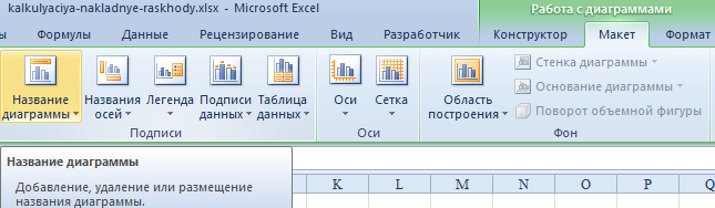
But you can safely do without a header. To remove it, you need to move it to an area of the graph that is invisible to prying eyes (above it). If you still need a chart title, you can access all the necessary settings through the “Chart Title” menu on the same tab. You can also find it under the Layout tab.
Instead of the serial number of the reporting year, it is enough to leave only the year itself. Select the desired values and right-click on them. Then click on “Select Data” – “Change Horizontal Axis Label”. Next, you need to set the range. In our case, this is the first column of the table that is the source of information. The result is this.
But in general, you can leave everything, this schedule is quite working. But if there is a need to make an attractive design of the chart, then the “Designer” tab is at your service, which allows you to specify the background color of the chart, its font, and also place it on another sheet.
Creating a Plot with Multiple Curves
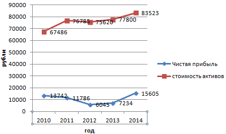
Suppose we need to demonstrate to investors not only the net profit of the enterprise, but also how much its assets will cost in total. Accordingly, the amount of information has increased.
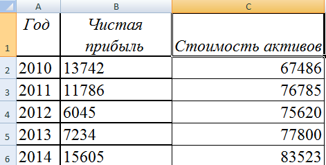
Despite this, there are no fundamental differences in the method of creating a graph compared to those described above. It’s just that now the legend should be left, because its function is perfectly performed.
Creating a second axis
What actions need to be taken to create another axis on the chart? If we use common metric units, then the tips described earlier must be applied. If different types of data are used, then one more axis will have to be added.
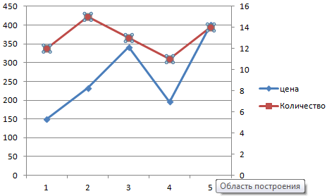
But before that, you need to build a regular graph, as if using the same metric units.
After that, the main axis is highlighted. Then call the context menu. There will be many items in it, one of which is “Data Series Format”. It needs to be pressed. Then a window will appear in which you need to find the menu item “Row Options”, and then set the option “Along the auxiliary axis”.
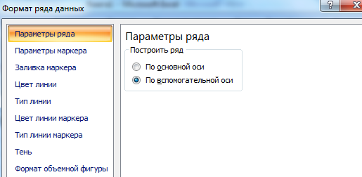
Next, close the window.
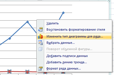
But this is just one of the possible methods. Nobody bothers, for example, to use a chart of a different kind for the secondary axis. We need to decide which line requires us to add an additional axis, and then right-click on it and select “Change Chart Type for Series”.
Next, you need to customize the “appearance” of the second row. We decided to stick with the bar chart.
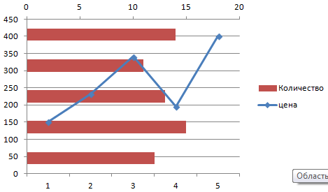
Here’s how simple it is. It is enough to make only a couple of clicks, and another axis appears, configured for a different parameter.
Excel: Technique for Creating a Graph of a Function
This is already a more non-trivial task, and in order to complete it, you need to perform two main steps:
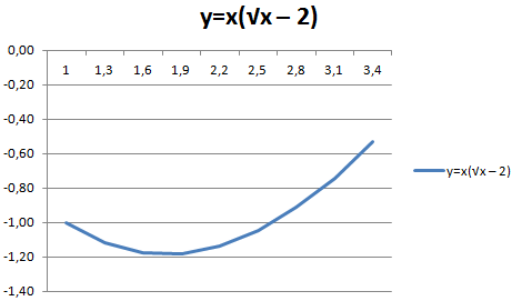
- Create a table that serves as a source of information. First you need to decide which function will be used specifically in your case. For example, y=x(√x – 2). In this case, we will choose the value 0,3 as the used step.
- Actually, build a graph.
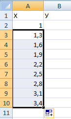
So, we need to form a table with two columns. The first is the horizontal axis (that is, X), the second is the vertical (Y). The second line contains the first value, in our case it is one. On the third line, you need to write a value that will be 0,3 more than the previous one. This can be done both with the help of independent calculations, and by writing the formula directly, which in our case will be as follows:
=A2+0,3.
After that, you need to apply autocomplete to the following cells. To do this, select cells A2 and A3 and drag the box to the required number of lines down.
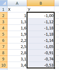
In the vertical column, we indicate the formula used to plot the function graph based on the finished formula. In the case of our example, this would be =A2*(ROOT(A2-2). After that, he confirms his actions with the Enter key, and the program will automatically calculate the result.
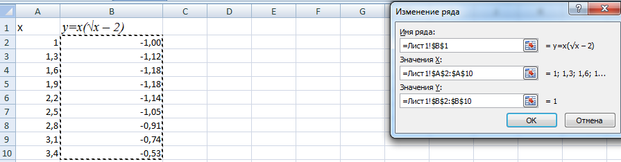
Next, you need to create a new sheet or switch to another, but already existing one. True, if there is an urgent need, you can insert a diagram here (without reserving a separate sheet for this task). But only on condition that there is a lot of free space. Then click the following items: “Insert” – “Chart” – “Scatter”.
After that, you need to decide what type of chart you want to use. Further, the right mouse click is made on that part of the diagram for which the data will be determined. That is, after opening the context menu, you should click on the “Select data” button.
Next, you need to select the first column, and click “Add”. A dialog box will appear, where there will be settings for the name of the series, as well as the values of the horizontal and vertical axes.
Hurray, the result is, and it looks very nice.
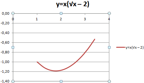
Similarly to the graph built at the beginning, you can delete the legend, since we have only one line, and there is no need to additionally label it.
But there is one problem – there are no values on the X-axis, only the number of points. To correct this problem, you need to name this axis. To do this, you need to right-click on it, and then select “Select Data” – “Change Horizontal Axis Labels”. Upon completion of these operations, the required set of values is selected, and the graph will look like this.
How to merge multiple charts
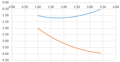
To create two graphs on the same field, you don’t need any special competencies. To start, you need to add the next column with the function Z=X(√x – 3).
To make it clearer, here is a table.
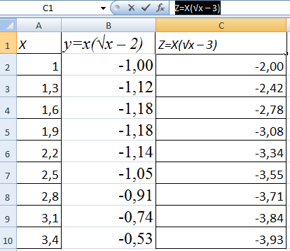
We find cells with the required information and select them. After that, they need to be inserted into the diagram. If something does not go according to plan (for example, wrong row names or wrong numbers on the axis were accidentally written), then you can use the “Select data” item and edit them. As a result, a graph like this will appear, where the two lines are combined together.
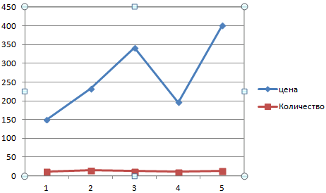
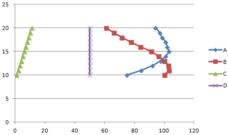
Dependency Plots
This is a type of graph where the content of one row or column directly affects the result of another. To create it, you need to form a plate like this one.
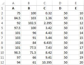
Schedule conditions: А = f (E); В = f (E); С = f (E); D = f (E).
In our case, we need to find a scatter plot with markers and smooth curves, since this type is most suitable for our tasks. Then click on the following buttons: Select data – Add. Let the row name be “A” and the X values be the A values. In turn, the vertical values will be the E values. Click “Add” again. The second row will be called B, and the values located along the X axis will be in column B, and along the vertical axis – in column E. Further, the entire table is created using this mechanism.
Customizing the Appearance of an Excel Graph
After the chart is created, you need to pay special attention to setting it up. It is important that its appearance is attractive. The principles of setting are the same, regardless of the version of the program used.
It is important to understand that any diagram is inherently a complex object. Therefore, it includes many smaller parts. Each of them can be configured by calling the context menu.
Here you need to distinguish between setting the general parameters of the chart and specific objects. So, to configure its basic characteristics, you need to click on the background of the diagram. After that, the program will show a mini-panel where you can manage the main general parameters, as well as various menu items where you can configure them more flexibly.
To set the background of the chart, you need to select the “Chart Area Format” item. If the properties of specific objects are adjusted, then the number of menu items will decrease significantly. For example, to edit the legend, simply call the context menu and click on the item there, which always begins with the word “Format”. You can usually find it at the very bottom of the context menu.
General guidelines for creating graphs
There are several recommendations on how to properly create graphs so that they are readable and informative:
- You don’t need to use too many lines. Just two or three is enough. If you need to display more information, it is better to create a separate graph.
- You need to pay special attention to the legend, as well as the axes. How well they are signed depends on how easy it will be to read the chart. This is important because any chart is created to simplify the presentation of certain information, but if approached irresponsibly, it will be harder for a person to understand.
- Although you can customize the appearance of the chart, it is not recommended to use too many colors. This will confuse the person reading the diagrams.
Conclusions
In simple words, it is absolutely easy to create a graph using a specific range of values as a data source. It is enough to press a couple of buttons, and the program will do the rest on its own. Of course, for professional mastery of this instrument, you need to practice a little.
If you follow the general recommendations for creating charts, as well as beautifully design the chart in such a way that you get a very beautiful and informative picture that will not cause difficulties when reading it.