Filter in Excel – Basics

Filtering data in Excel allows you to display among a large amount of information only what you currently need. For example, having a list of thousands of goods in a large hypermarket in front of you, you can select only shampoos or creams from it, and temporarily hide the rest. In this lesson, we will learn how to apply filters to lists in Excel, set filtering on several columns at once, and remove filters.

If your table contains a large amount of data, it may be difficult to find the information you need. Filters are used to narrow down the amount of data displayed on an Excel sheet, allowing you to see only the information you need.

Applying a filter in Excel

In the following example, we will apply a filter to the hardware usage log to display only laptops and tablets available for review.

1. Select any cell in the table, for example cell A2.

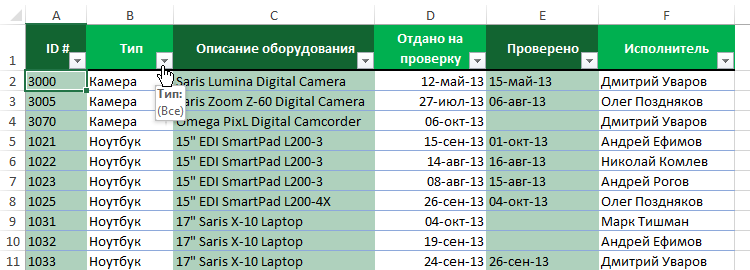
For filtering to work correctly in Excel, the worksheet must contain a header row that is used to name each column. In the following example, the data on the worksheet is organized as columns with headings on row 1: ID #, Type, Hardware Description, and so on.

1. Click the Data, then press command Filter.
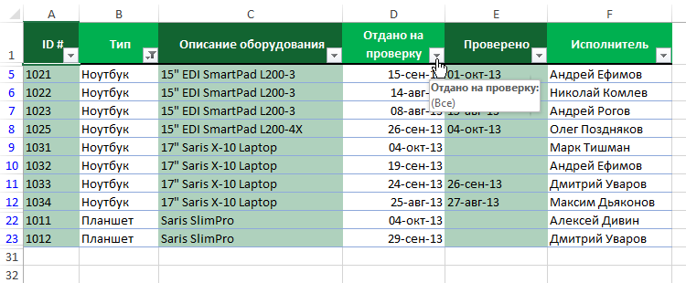
2. Arrow buttons appear in the headings of each column.
3. Click on such a button in the column you want to filter. In our case, we will apply a filter to column B to see only the types of equipment we need.
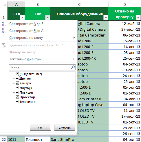
4. The filter menu will appear.
5. Uncheck the box Select allto quickly deselect all items.
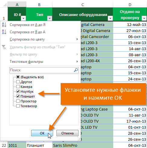
6. Check the boxes for the types of equipment you want to leave in the table, then click OK. In our example, we will choose Laptops и Tabletsto see only those types of equipment.
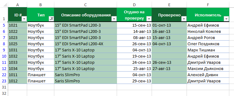
7. The data table will be filtered, temporarily hiding all content that does not match the criteria. In our example, only laptops and tablets remained visible.

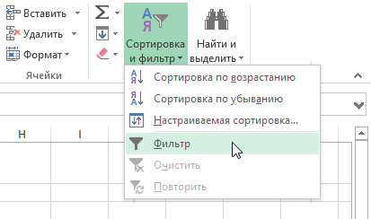
Filtering can also be applied by selecting the command Sort and filter tab Home.

Apply multiple filters in Excel

Filters in Excel can be summed up. This means that you can apply multiple filters to the same table to narrow down the filter results. In the previous example, we already filtered the table to display only laptops and tablets. Now our task is to narrow down the data even more and show only laptops and tablets submitted for review in August.

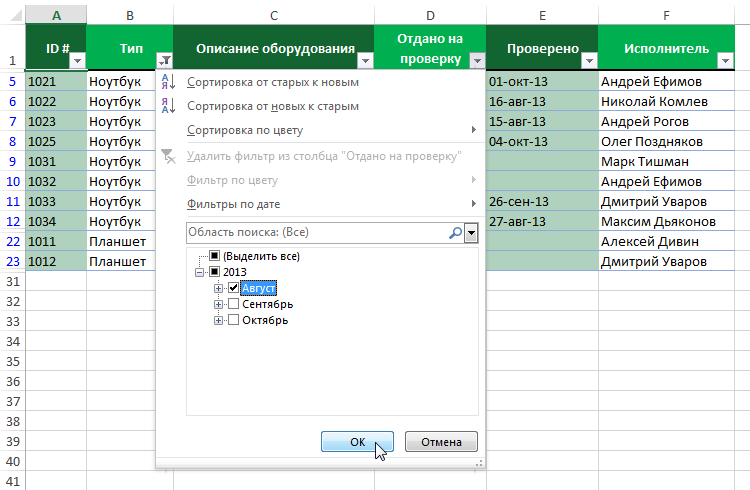
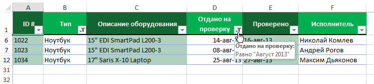
1. Click the arrow button in the column you want to filter. In this case, we’ll apply an additional filter to column D to see information by date.
2. The filter menu will appear.
3. Check or uncheck the boxes depending on the data you want to filter, then click OK. We will deselect all items except August.
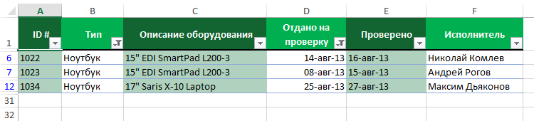
4. The new filter will be applied, and only laptops and tablets that were submitted for verification in August will remain in the table.

Removing a filter in Excel

After applying the filter, sooner or later it will be necessary to remove or remove it in order to filter the content in a different way.

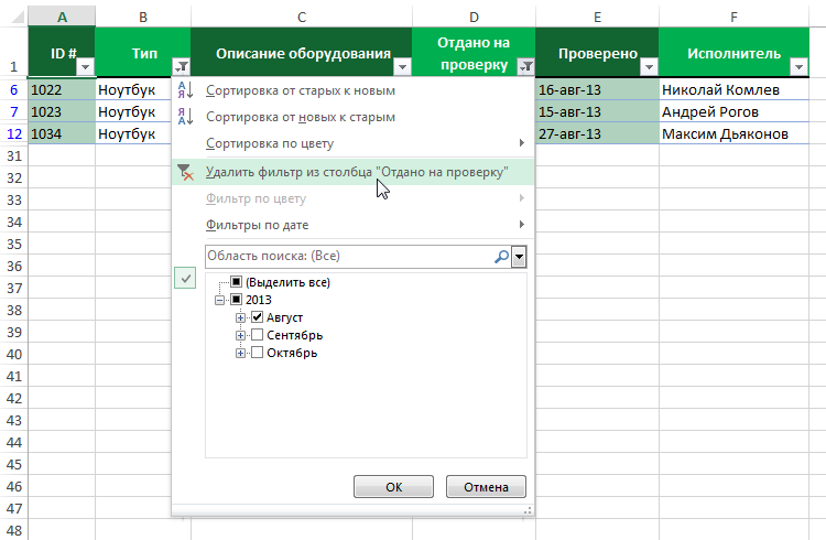
1. Click the arrow button in the column you want to remove the filter from. In our example, we will remove the filter from column D.
2. The filter menu will appear.
3. Select item Remove filter from column… In our example, we will remove the filter from the column Submitted for review.
4. The filter will be removed and the previously hidden data will reappear in the Excel sheet.

To remove all filters in an Excel table, click the command Filter tab Data.