Division in Excel. How division works in Excel

Excel is an incredibly functional program. It can be used both as a kind of programming environment and as a very functional calculator that allows you to calculate anything. Today we will look at the second application of this application, namely the division of numbers.

This is one of the most common uses of spreadsheets, along with other arithmetic operations such as addition, subtraction, and multiplication. In fact, division must be carried out in almost any mathematical operation. It is also used in statistical calculations, and for this this spreadsheet processor is used very often.

Division capabilities in an Excel spreadsheet

In Excel, you can bring several basic tools at once to carry out this operation, and today we will give those that are used most often. This is the use of formulas with direct indication of values ​​​​(which are numbers or addresses of cells) or the use of a special function to perform this arithmetic operation.

Dividing a number by a number

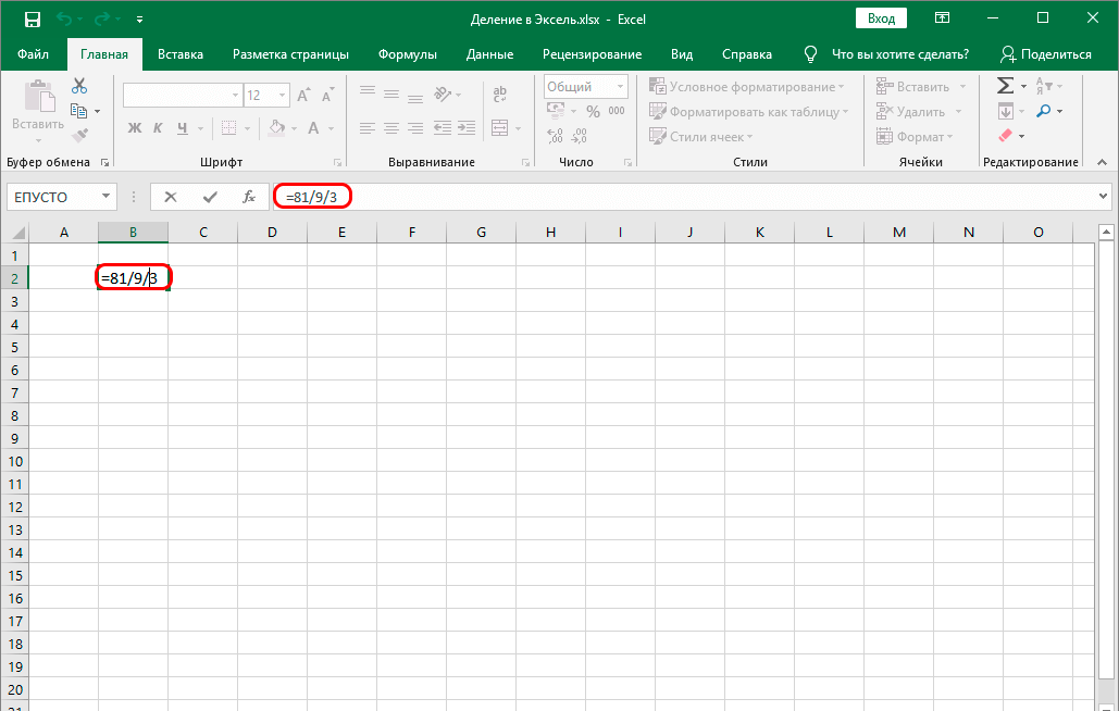
This is the most elementary way to do this mathematical operation in Excel. It is performed in the same way as on a conventional calculator that supports the input of mathematical expressions. The only difference is that before entering numbers and signs of arithmetic operators, you must enter the = sign, which will show the program that the user is about to enter a formula. To carry out the division operation, you must use the / sign. Let’s see how this works in practice. To do this, follow the steps described in this manual:

1. We carry out a mouse click on any cell that does not contain any data (including formulas that give an empty result or non-printable characters).
2. Input can be done in several ways. You can directly start typing the necessary characters, starting with the equal sign, and there is an opportunity to enter the formula directly into the formula input line, which is located above.
3. In any case, you must first write the = sign, and then write the number to be divided. After that, we put a slash symbol, after which we manually write down the number by which the division operation will be carried out.
4. If there are several divisors, they can be added to each other using additional slashes.
5. To record the result, you must press the key Enter. The program will automatically perform all the necessary calculations.

Now we check whether the program has written the correct value. If the result turns out to be wrong, there is only one reason – the wrong formula entry. In this case, you need to correct it. To do this, click on the appropriate place in the formula bar, select it and write down the value that is correct. After that, press the enter key, and the value will be automatically recalculated.

Other operations may also be used to perform mathematical operations. They can be combined with division. In this case, the procedure will be as it should be according to the general rules of arithmetic:

1. The operation of division and multiplication is performed first. Addition and subtraction come second.
2. Expressions can also be enclosed in parentheses. In this case, they will take precedence, even if they contain addition and subtraction operations.

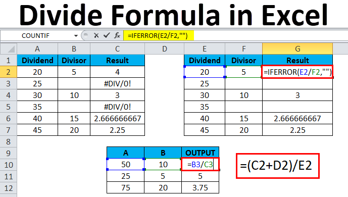
We all know that, according to the basic mathematical laws, division by zero is impossible. And what will happen if we try to carry out a similar operation in Excel? In this case, the error “#DIV/0!” will be issued.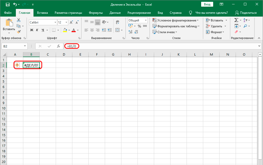

Cell data division

We are slowly making things harder. What if, for example, we need to separate cells among themselves? Or if you need to divide the value contained in a certain cell by a certain number? I must say that the standard features of Excel provide such an opportunity. Let’s take a closer look at how to do this.

1. We make a click on any cell that does not contain any values. Just like in the previous example, you need to make sure that there are no non-printable characters.
2. Next, enter the formula input sign =. After that, we left-click on the cell that contains the appropriate value.
3. Then enter the division symbol (slash).
4. Then again select the cell that you want to split. Then, if required, enter the slash again and repeat steps 3-4 until the proper number of arguments is entered.
5. After the expression has been fully entered, press Enter to show the result in the table.

If you need to divide the number by the contents of the cell or the contents of the cell by the number, then this can also be done. In this case, instead of clicking the left mouse button on the corresponding cell, you must write down the number that will be used as a divisor or dividend. You can also enter cell addresses from the keyboard instead of numbers or mouse clicks.

Dividing a column by a column

Excel allows you to perform the operation of dividing one column by another. That is, the numerator of one column will be divided by the denominator of the column next to it. It doesn’t take much time to do this, because the way this operation is done is a bit different, much faster than simply dividing each expression into each other. What needs to be done?

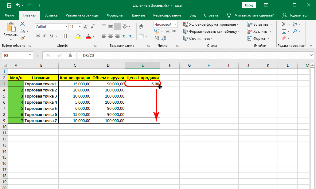
1. Click on the cell where the first final result will be displayed. After that, enter the formula input symbol =.
2. After that, left-click on the first cell, and then divide it into the second in the way that was described above.
3. Then press the enter key.

After performing this operation, the value will appear in the corresponding cell. So far everything is as described above.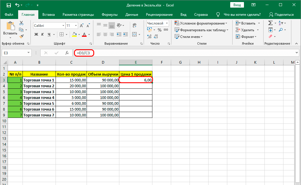

After that, you can perform the same operations on the following cells. But this is not the most efficient idea. It is much better to use a special tool called an autocomplete marker. This is a square that appears in the lower right corner of the selected cell. To use it, you need to move the mouse cursor over it. The fact that everything is done correctly can be found by changing the arrow to a cross. After that, press the left mouse button and holding it down, drag the formula to all the remaining cells.

After performing this operation, we get a column completely filled with the necessary data.

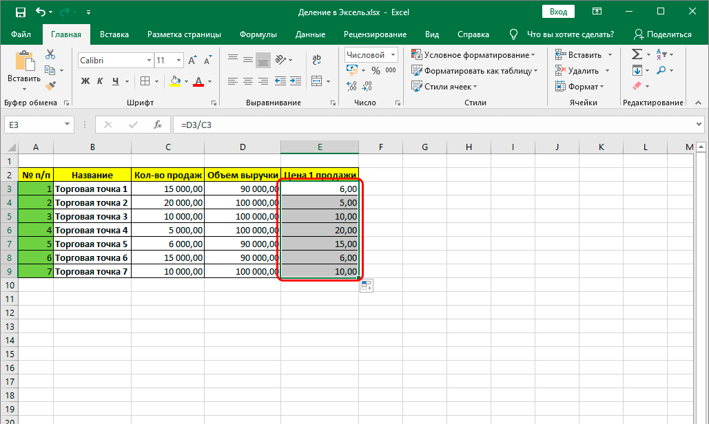
Attention. You can only move a formula in one direction with the AutoComplete handle. You can transfer values ​​both from bottom to top and from top to bottom. In this case, the cell addresses will be automatically replaced with the following ones.

This mechanism allows you to make the correct calculations in the following cells. However, if you need to split a column by the same value, this method will behave incorrectly. This is because the value of the second number will constantly change. Therefore, you need to use the fourth method in order for everything to be correct – dividing the column by a constant (constant number). But in general, this tool is very convenient to use if the column contains a huge number of rows.

Splitting a column into a cell

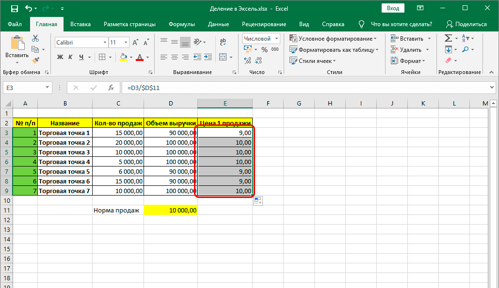
So, what should be done to divide an entire column by a constant value? To do this, you need to talk about two types of addresses: relative and absolute. The first ones are those described above. As soon as the formula is copied or moved to another location, the relative links are automatically changed to the appropriate ones.

Absolute references, on the other hand, have a fixed address and do not change when transferring a formula using a copy-paste operation or an auto-complete marker. What needs to be done in order to divide the whole column into one specific cell (for example, it may contain the amount of a discount or the amount of revenue for one product)?

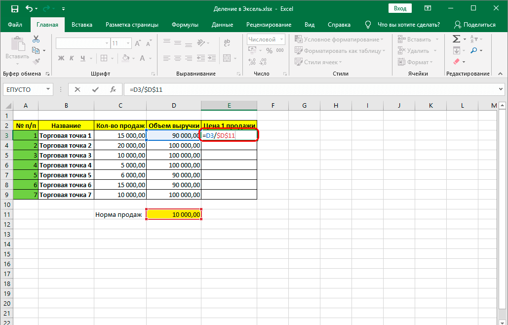
1. We make a left mouse click on the first cell of the column in which we will display the results of the mathematical operation. After that, we write down the input sign formula, click on the first cell, the division sign, the second, and so on according to the scheme. After that, we enter a constant, which will serve as the value of a particular cell.
2. Now you need to fix the link by changing the address from relative to absolute. We make a mouse click on our constant. After that, you need to press the F4 key on the computer keyboard. Also, on some laptops, you need to press the Fn + F4 button. To understand whether you need to use a specific key or combination, you can experiment or read the official documentation of the laptop manufacturer. After we press this key, we will see that the address of the cell has changed. Added a dollar sign. He tells us that the absolute address of the cell is used. You need to make sure that the dollar sign is placed next to both the letter for the column and the number for the row. If there is only one dollar sign, then the fixing will be carried out only horizontally or only vertically.
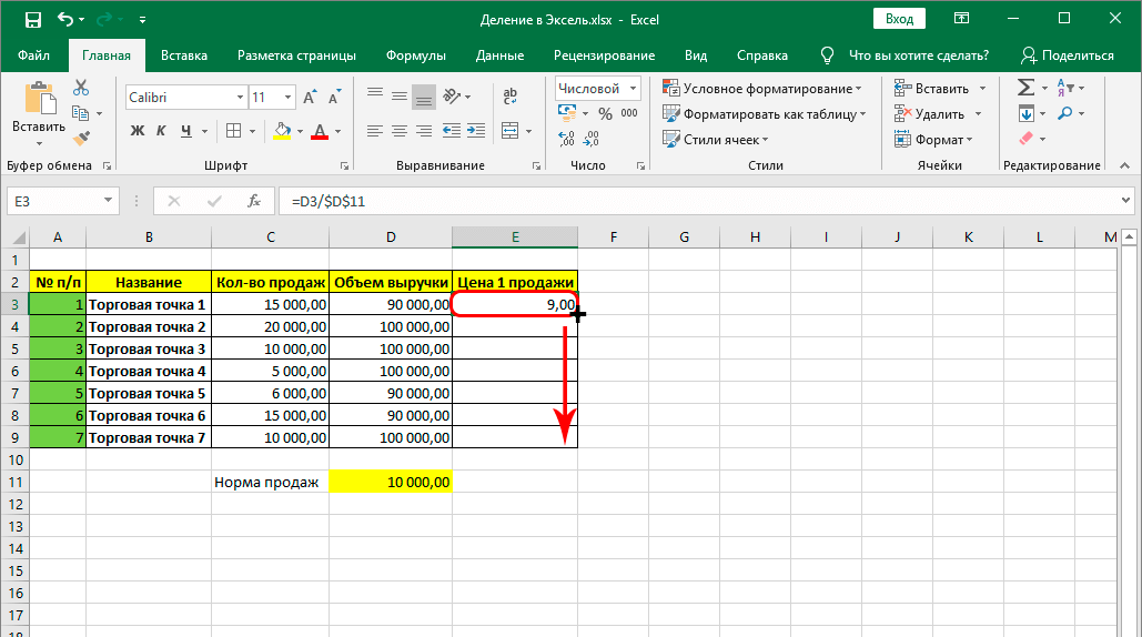
3. Next, to confirm the result, press the enter key, and then use the autofill marker to perform this operation with other cells in this column.
4. We see the result.

How to use the PRIVATE function

There is another way to perform division – using a special function. Its syntax is: =PARTIAL(numerator, denominator). It is impossible to say that it is better than the standard division operator in all cases. The fact is that it rounds the remainder to a smaller number. That is, the division is carried out without a remainder. For example, if the result of calculations using the standard operator (/) is the number 9,9, then after applying the function PRIVATE the value 9 will be written to the cell. Let’s describe in detail how to use this function in practice:

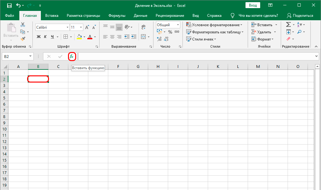
1. Click on the cell where the result of the calculations will be recorded. After that, open the insert function dialog box (to do this, click on the “Insert function” button, which is located immediately to the left next to the formula input line). This button looks like two latin letters fx.
2. After the dialog box appears, you need to open the complete alphabetical list of functions, and at the end of the list there will be an operator PRIVATE. We choose it. Just below it will be written what it means. Also, the user can read a detailed description of how to use this function by clicking on the “Help for this function” link. After completing all these steps, confirm your choice by pressing the OK button.
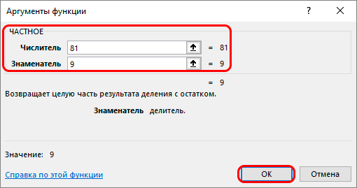
3. Another window will open in front of us, in which you need to enter the numerator and denominator. You can write down not only numbers, but also links. Everything is the same as with manual division. We check how correctly the data was indicated, and then confirm our actions.

Now we check if all the parameters were entered correctly. Life hack, you can not call the function input dialog box, but simply use the formula input line, writing the function there as =PRIVATE(81), as shown in the screenshot below. The first number is the numerator and the second is the denominator.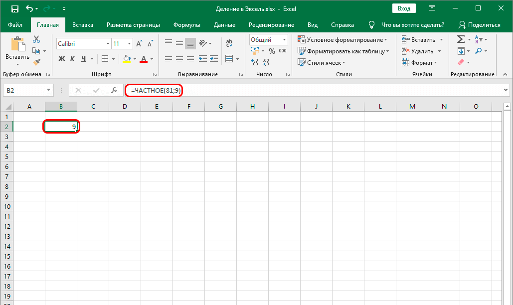

Function arguments are separated by semicolons. If the formula was entered incorrectly, you can correct it by making adjustments to the formula input line. So, today we have learned how to perform the division operation in different ways in Excel. There is nothing complicated in this, as we see. To do this, you need to use the division operator or the function PRIVATE. The first calculates the value in exactly the same way as a calculator. The second one can find a number without a remainder, which can also be useful in calculations.

Be sure to practice before using these functions in real practice. Of course, there is nothing complicated in these actions, but that a person has learned something can only be said when he performs the correct actions automatically, and makes decisions intuitively.