Calculating Confidence Interval in Excel

Excel is used to perform various statistical tasks, one of which is the calculation of the confidence interval, which is used as the most appropriate replacement for a point estimate with a small sample size.

We want to note right away that the very procedure for calculating the confidence interval is rather complicated, however, in Excel there are a number of tools designed to facilitate this task. Let’s take a look at them.

Confidence Interval Calculation

A confidence interval is needed in order to give an interval estimate to some static data. The main purpose of this operation is to remove the uncertainties of the point estimate.

There are two methods for performing this task in Microsoft Excel:

• Operator CONFIDENCE NORM – used in cases where the dispersion is known;
• Operator TRUST.STUDENTwhen the variance is unknown.

Below we will step by step analyze both methods in practice.

Method 1: TRUST.NORM statement

This function was first introduced into the arsenal of the program in the Excel 2010 edition (before this version, it was replaced by the operator “TRUSTED”). The operator is included in the “statistical” category.

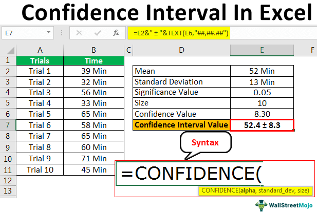
Function Formula CONFIDENCE NORM looks like that:

=ДОВЕРИТ.НОРМ(Альфа;Станд_откл;Размер)

As we can see, the function has three arguments:

• “Alpha” is an indicator of the level of significance, which is taken as the basis for the calculation. The confidence level is calculated as follows:
  • 1-"Альфа". This expression is applicable if the value “Alpha” presented as a coefficient. For example, 1-0,7 0,3 =, where 0,7=70%/100%.
  • (100-"Альфа")/100. This expression will be applied if we consider the confidence level with the value “Alpha” in percents. For example, (100-70) / 100 = 0,3.
• “Standard deviation” – respectively, the standard deviation of the analyzed data sample.
• “Size” is the size of the data sample.

Note: For this function, the presence of all three arguments is a prerequisite.

Operator “TRUSTED”, which was used in earlier versions of the program, contains the same arguments and performs the same functions.

Function Formula TRUSTED as follows:

=ДОВЕРИТ(Альфа;Станд_откл;Размер)

There are no differences in the formula itself, only the name of the operator is different. In Excel 2010 and later editions, this operator is in the Compatibility category. In older versions of the program, it is located in the static functions section.

The confidence interval boundary is determined by the following formula:

X+(-)ДОВЕРИТ.НОРМ

where Х is the average value over the specified range.

Now let’s see how to apply these formulas in practice. So, we have a table with various data from 10 measurements taken. In this case, the standard deviation of the data set is 8.

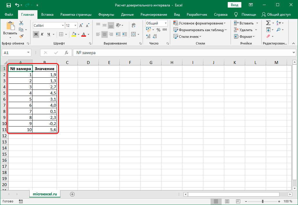
Our task is to obtain the value of the confidence interval with a 95% confidence level.

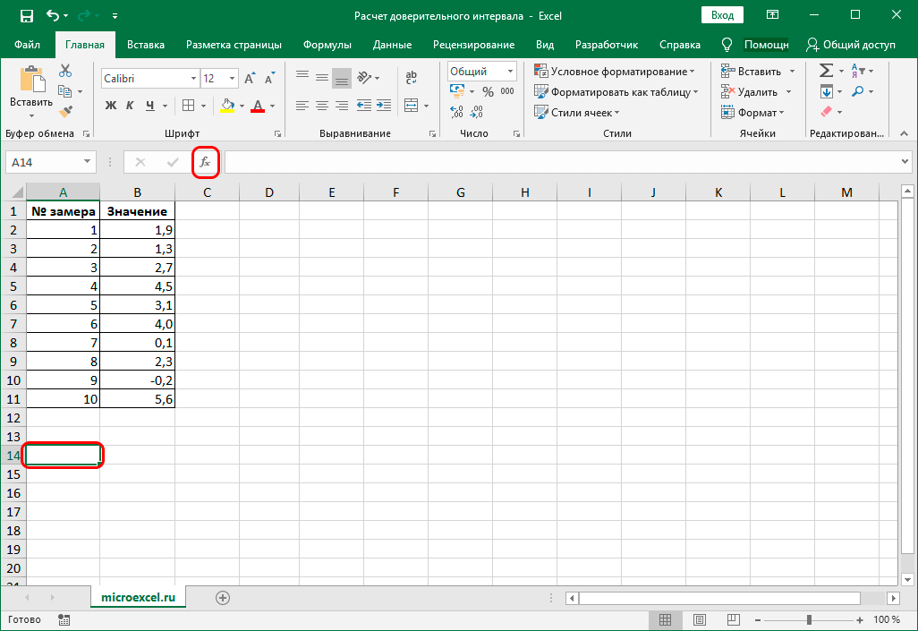
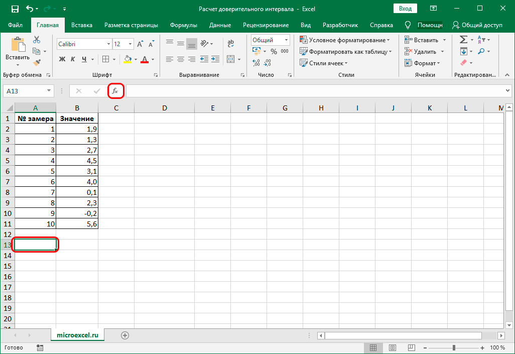
1. First of all, select a cell to display the result. Then we click on the button “Insert function” (to the left of the formula bar).
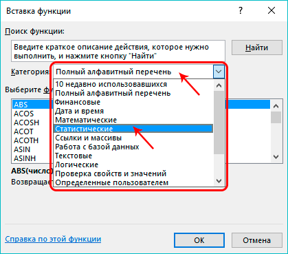
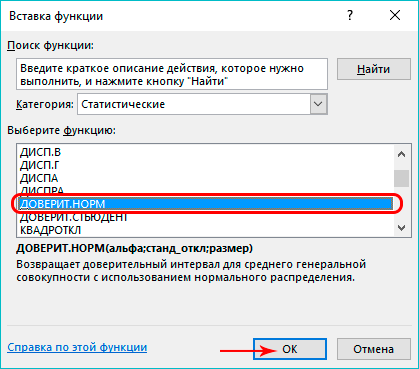
2. The Function Wizard window opens. By clicking on the current category of functions, expand the list and click on the line in it “Statistical”.
3. In the proposed list, click on the operator “CONFIDENCE NORM”, then press OK.
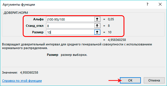
4. We will see a window with the settings of the function arguments, filling which we press the button OK.
   • in the field “Alpha” indicate the level of significance. Our task assumes a 95% confidence level. Substituting this value into the calculation formula, which we considered above, we obtain the expression: (100-95)/100. We write it in the argument field (or you can immediately write the result of the calculation equal to 0,05).
   • in the field “std_off” according to our conditions, we write the number 8.
   • in the “Size” field, specify the number of elements to be examined. In our case, 10 measurements were taken, so we write the number 10.
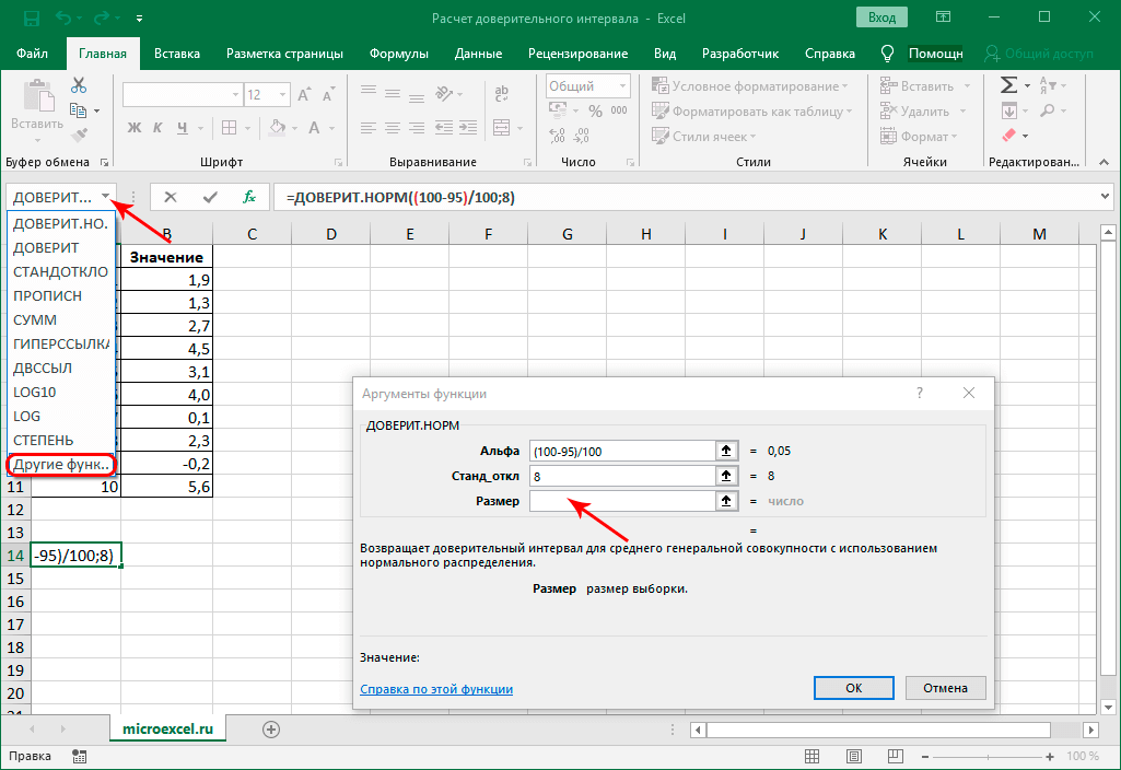
5. To avoid having to reconfigure the function when data changes, you can automate it. For this we use the function “CHECK”. Put the pointer in the input area of ​​the argument information “Size”, then click on the triangle icon on the left side of the formula bar and click on the item “More features…”.
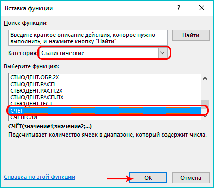
6. As a result, another window of the Function Wizard will open. By choosing a category “Statistical”, click on the function “CHECK”, then OK.
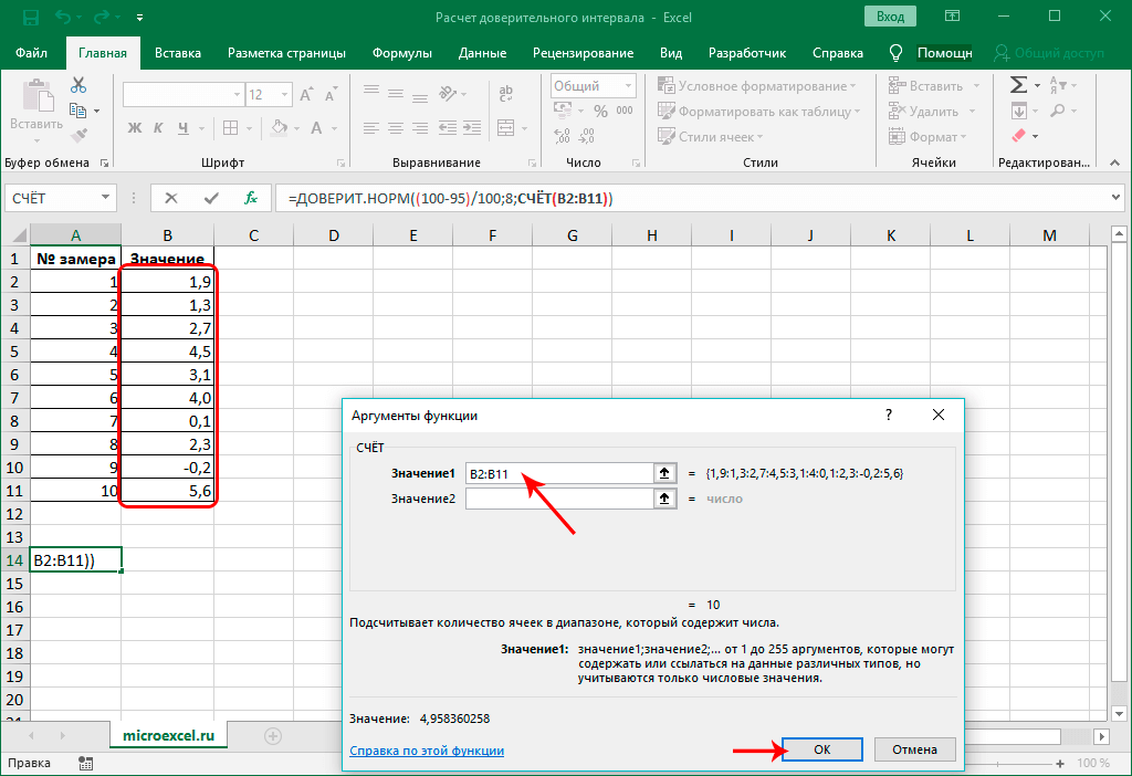
7. The screen will display another window with the settings of the arguments of the function, which is used to determine the number of cells in a given range that contain numeric data.

   Function Formula CHECK it is written like this: =СЧЁТ(Значение1;Значение2;...).

   The number of available arguments for this function can be up to 255. Here you can write either specific numbers, or cell addresses, or cell ranges. We will use the last option. To do this, click on the information input area for the first argument, then, holding down the left mouse button, select all the cells of one of the columns of our table (not counting the header), and then press the button OK.

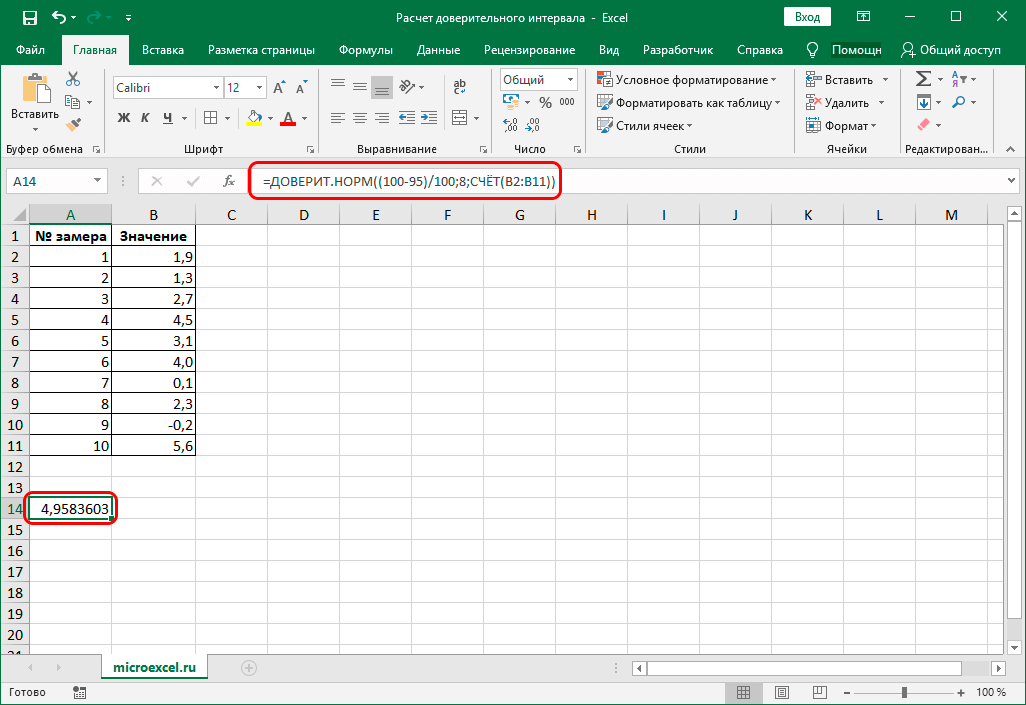
8. As a result of the actions taken, the result of calculations for the operator will be displayed in the selected cell CONFIDENCE NORM. In our problem, its value turned out to be equal to 4,9583603.
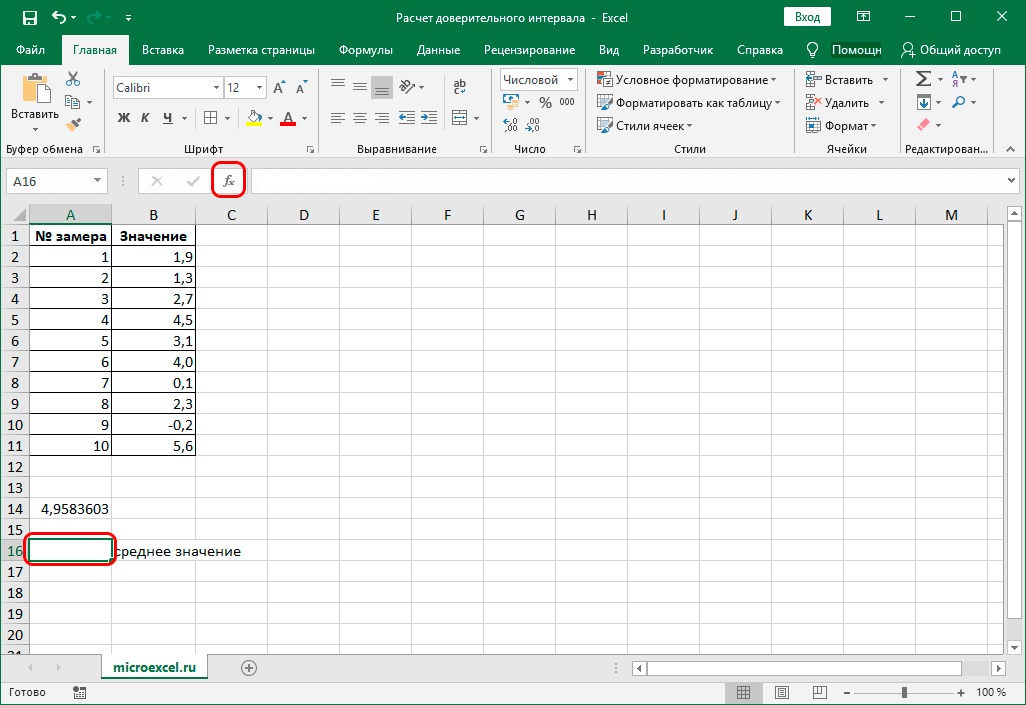
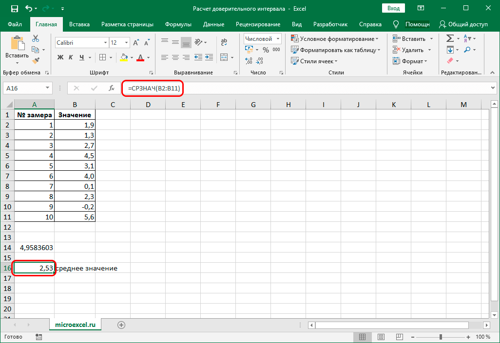
9. But this is not yet the final result in our task. Next, you need to calculate the average value over a given interval. To do this, you need to use the function “HEART”A that performs the task of calculating the average over a specified range of data.

   The operator formula is written like this: =СРЗНАЧ(число1;число2;...).

   Select the cell where we plan to insert the function and press the button “Insert function”.

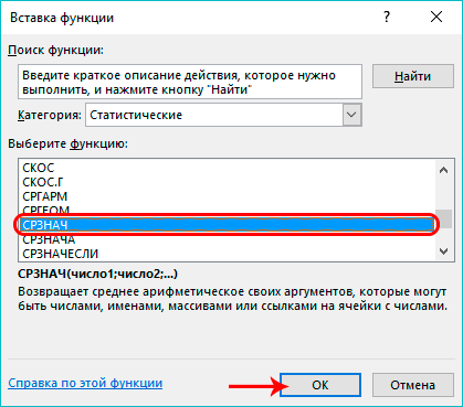
10. In category “Statistical” choose a boring operator “HEART” and click OK.
11. In function arguments in argument value “Number” specify the range, which includes all cells with the values ​​of all measurements. Then we click OKAY.
12. As a result of the actions taken, the average value will be automatically calculated and displayed in the cell with the newly inserted function.
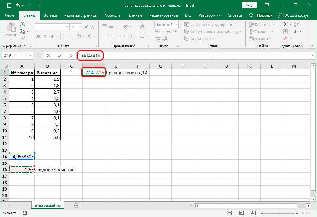
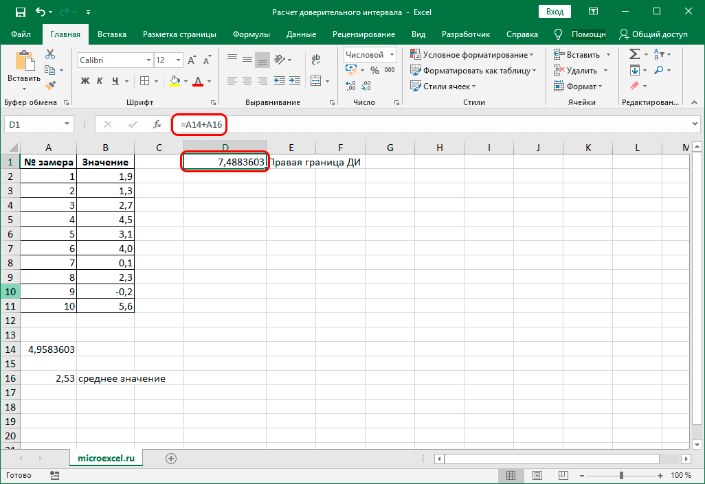
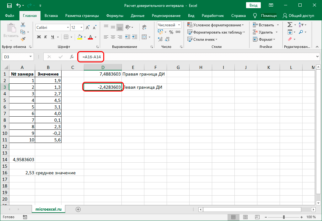
13. Now we need to calculate the CI (confidence interval) bounds. Let’s start by calculating the value of the right border. We select the cell where we want to display the result, and perform the addition of the results obtained using the operators “HEART” and “CONFIDENCE NORMS”. In our case, the formula looks like this: A14+A16. After typing it, press Enter.
14. As a result, the calculation will be performed and the result will be immediately displayed in the cell with the formula.
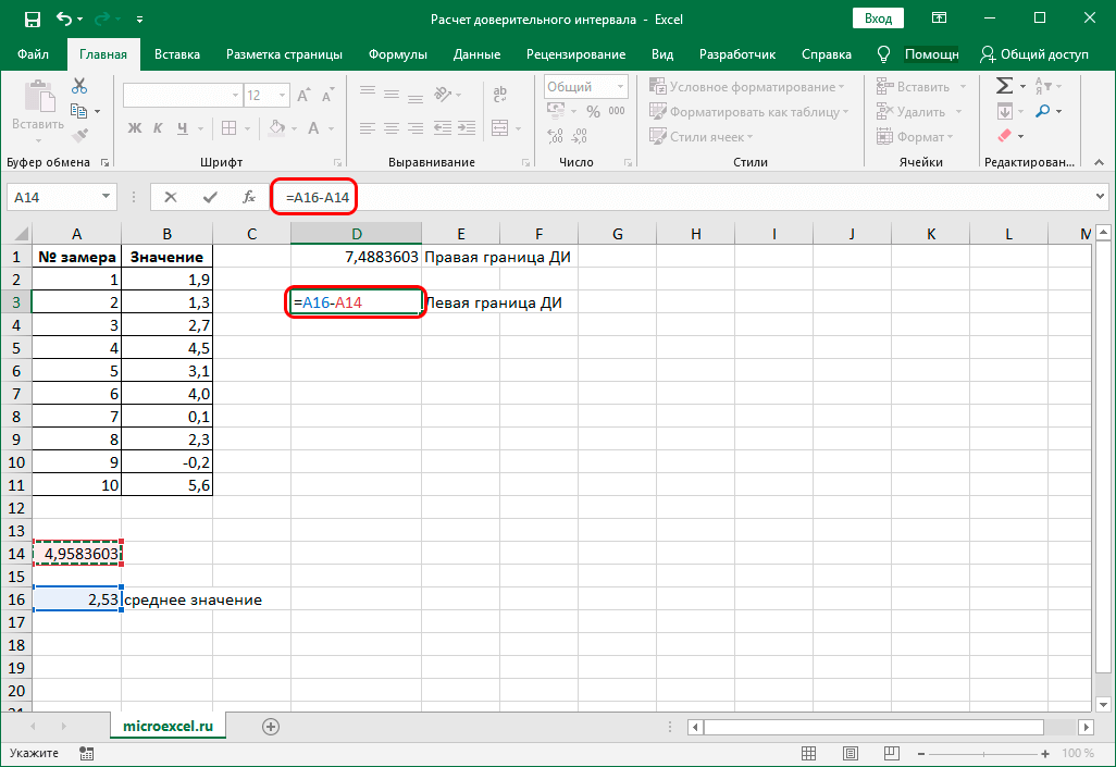
15. Then, in a similar way, we perform the calculation to obtain the value of the left border of the CI. Only in this case the value of the result “CONFIDENCE NORMS” you do not need to add, but subtract from the result obtained using the operator “HEART”. In our case, the formula looks like this: =A16-A14.
16. After pressing Enter, we will get the result in the given cell with the formula.

Note: In the paragraphs above, we tried to describe in as much detail as possible all the steps and each function used. However, all the prescribed formulas can be written together, as part of one large one:

• To determine the right border of the CI, the general formula will look like this:

  =СРЗНАЧ(B2:B11)+ДОВЕРИТ.НОРМ(0,05;8;СЧЁТ(B2:B11)).

• Similarly, for the left border, only instead of a plus, you need to put a minus:

  =СРЗНАЧ(B2:B11)-ДОВЕРИТ.НОРМ(0,05;8;СЧЁТ(B2:B11)).

Method 2: TRUST.STUDENT operator

Now, let’s get familiar with the second operator for determining the confidence interval − TRUST.STUDENT. This function was introduced into the program relatively recently, starting from the version of Excel 2010, and is aimed at determining the CI of the selected dataset using the Student’s distribution, with an unknown variance.

Function Formula TRUST.STUDENT as follows:

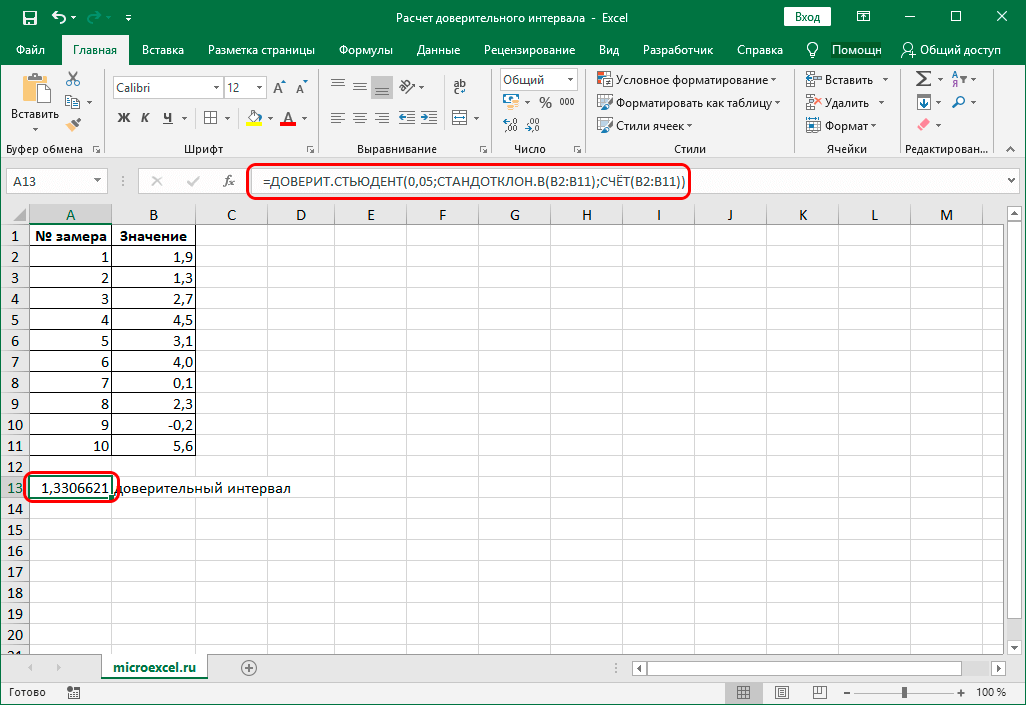
=ДОВЕРИТ.СТЬЮДЕНТ(Альфа;Cтанд_откл;Размер)

Let’s analyze the application of this operator on the example of the same table. Only now we do not know the standard deviation according to the conditions of the problem.

1. First, select the cell where we plan to display the result. Then click on the icon “Insert function” (to the left of the formula bar).
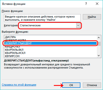
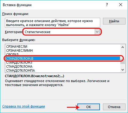
2. The already well-known Function Wizard window will open. Choose a category “Statistical”, then from the proposed list of functions, click on the operator “TRUSTED STUDENT”, then – OK.
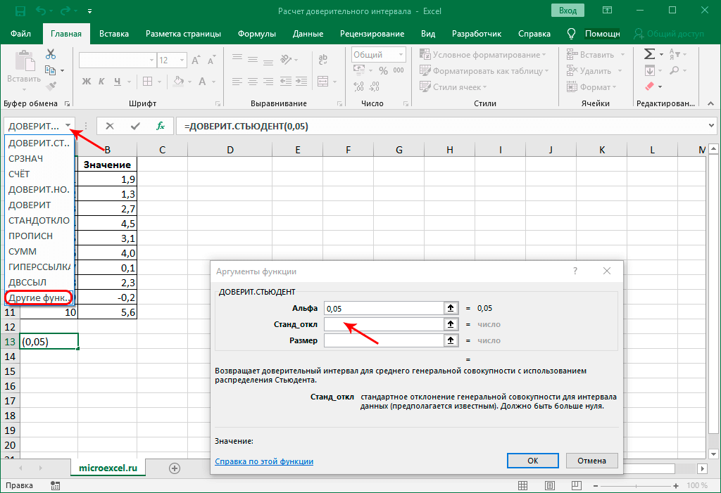
3. In the next window, we need to set up the function arguments:
   • In the “Alpha” as in the first method, specify the value 0,05 (or “100-95)/100”).
   • Let’s move on to the argument. “std_off”. Because according to the conditions of the problem, its value is unknown to us, we need to make the appropriate calculations, in which the operator “STDEV.B”. Click on the add function button and then on the item “More features…”.
   • In the next window of the Function Wizard, select the operator “STDEV.B” in category “Statistical” and click OK.
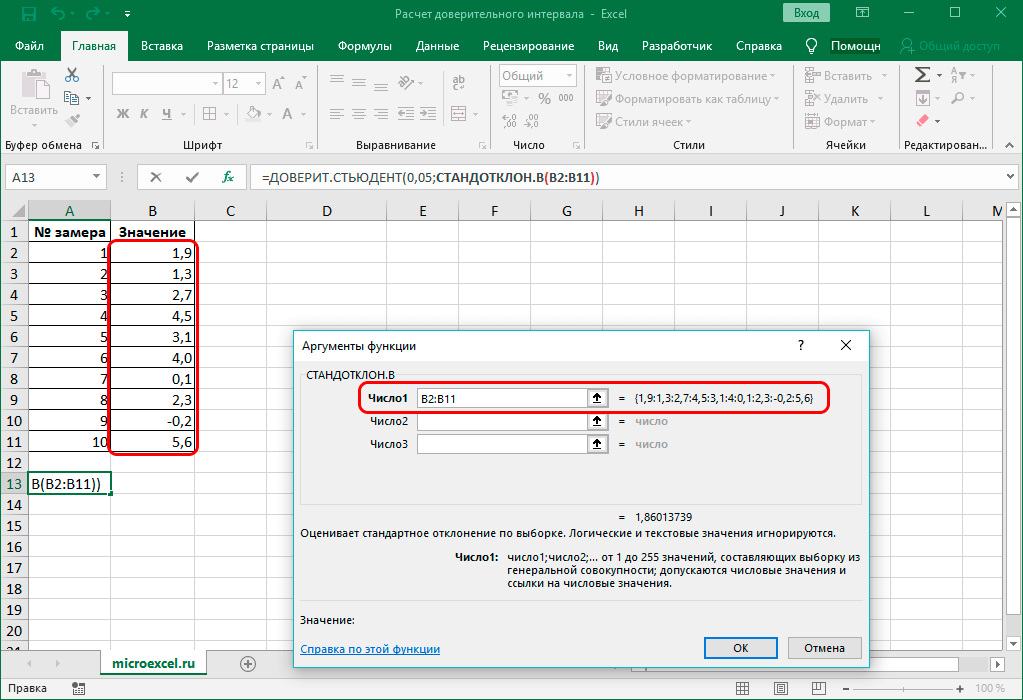
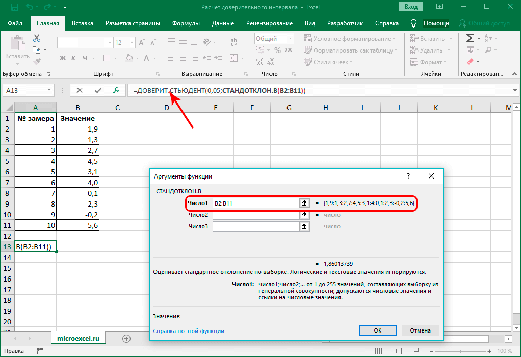
   • We get into the function arguments settings window, the formula of which looks like this: =СТАНДОТКЛОН.В(число1;число2;...). As the first argument, we specify a range that includes all cells in the “Value” column (not counting the header).
   • Now you need to go back to the window with the function arguments “TRUST.STUDENT”. To do this, click on the inscription of the same name in the formula input field.
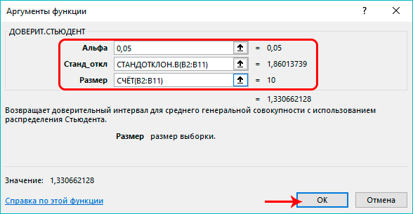
   • Now let’s move on to the last argument “Size”. As in the first method, here you can either simply specify a range of cells, or insert the operator “CHECK”. We choose the last option.
   • Once all the arguments are filled in, click the button OK.
4. The selected cell will display the value of the confidence interval according to the parameters we specified.
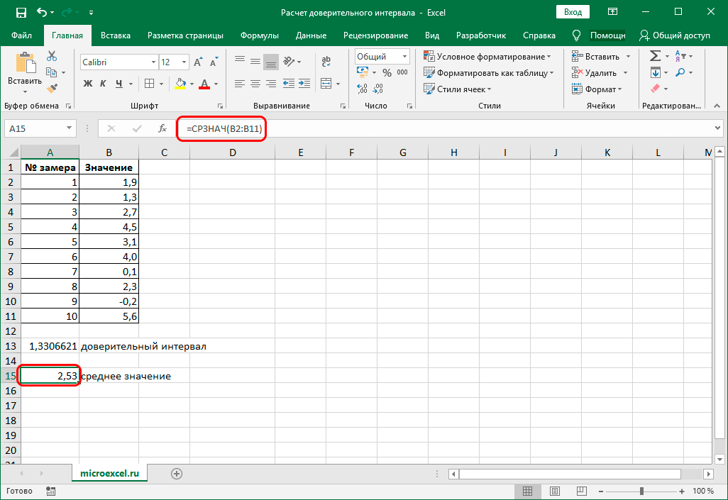
5. Next, we need to calculate the values ​​of the CI boundaries. And for this you need to get the average value for the selected range. To do this, we again apply the function “HEART”. The algorithm of actions is similar to that described in the first method.
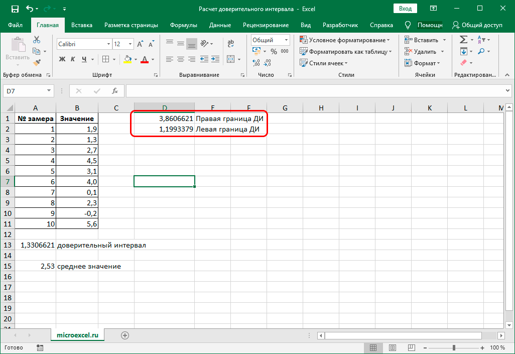
6. Having received the value “HEART”, you can start calculating the CI boundaries. The formulas themselves are no different from those used with the “CONFIDENCE NORMS”:
   • Right border CI=AVERAGE+STUDENT CONFIDENCE
   • Left Bound CI=AVERAGE-STUDENT CONFIDENCE

Conclusion

Excel’s arsenal of tools is incredibly large, and along with common functions, the program offers a wide variety of special functions that will make working with data much easier. Perhaps the steps described above may seem complicated to some users at first glance. But after a detailed study of the issue and the sequence of actions, everything will become much easier.