


Contents
If you often build reports with financial indicators (KPI) in Excel, then you should like this exotic type of chart – a scale chart or a thermometer chart (Bullet Chart):
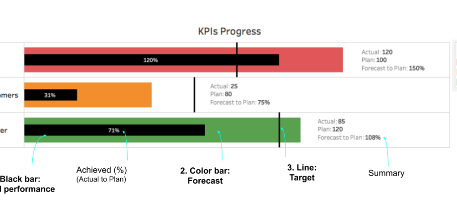
- The horizontal red line shows the target value we are aiming for.
- The three-color background fill of the scale clearly displays the “bad-medium-good” zones where we get.
- The black center rectangle displays the current value of the parameter.
Of course, there are no previous values of the parameter in such a diagram, i.e. We will not see any dynamics or trends, but for a pinpoint display of the achieved results vs goals at the moment, it is quite suitable.
Video
Stage 1. Stacked histogram
We will have to start by building a standard histogram based on our data, which we will then bring to the form we need in a few steps. Select the source data, open the tab Insert and choose stacked histogram:


Now we add:
- To make the columns line up not in a row, but on top of each other, swap the rows and columns using the button Row/Column (Row/Column) tab Constructor (Design).
- We remove the legend and the name (if any) – we have minimalism here.
- Adjust the color fill of the columns according to their meaning (select them one by one, right-click on the selected one and select Data point format).
- Narrowing the chart in width
The output should look something like this:

Stage 2. Second axis
Select a row Value (black rectangle), open its properties with a combination Ctrl + 1 or right click on it — Row Format (Format Data Point) and in the parameters window switch the row to Auxiliary axis (Secondary Axis).

The black column will go along the second axis and begin to cover all the other colored rectangles – don’t be scared, everything is according to the plan 😉 To see the scale, increase for it Side clearance (Gap) to the maximum to get a similar picture:

It’s already warmer, isn’t it?
Stage 3. Set a goal
Select a row Goal (red rectangle), right-click on it, select the command Change chart type for a series and change the type to Dotted (Scatter). The red rectangle should turn into a single marker (round or L-shaped), i.e. exactly:

Without removing the selection from this point, turn on for it Error Bars tab Layout. or on the tab Constructor (in Excel 2013). The latest versions of Excel offer several options for these bars – experiment with them if you wish:


From our point, “whiskers” should diverge in all four directions – they are usually used to visually display accuracy tolerances or scatter (dispersion) of values, for example, in statistics, but now we use them for a more prosaic purpose. Delete the vertical bars (select and press the key Delete), and adjust the horizontal ones by right-clicking on them and selecting the command Format Error Bars:

In the properties window of horizontal bars of errors in the section Error value Choose fixed value or Custom (Custom) and set the positive and negative value of the error from the keyboard equal to 0,2 – 0,5 (selected by eye). Here you can also increase the thickness of the bar and change its color to red. The marker can be disabled. As a result, it should turn out like this:

Stage 4. Finishing touches
Now there will be magic. Watch your hands: select the right additional axis and press Delete on keyboard. All our constructed scale columns, the target error bar and the main black rectangle of the current parameter value are reduced to one coordinate system and begin to be plotted along one axis:

That’s it, the diagram is ready. Beautiful, is not it? 🙂
Most likely you will have several parameters that you want to display using such charts. In order not to repeat the whole saga with the construction, you can simply copy the chart, and then (selecting it) drag the blue rectangle of the source data zone to new values:

- How to build a Pareto chart in Excel
- How to build a waterfall chart of deviations (“waterfall” or “bridge”) in Excel
- What’s New in Charts in Excel 2013