30 Excel functions in 30 days: INDEX

Yesterday in the marathon 30 Excel functions in 30 days we searched for text strings using the function FIND (FIND), and found out that it is case sensitive, unlike the function SEARCH (SEARCH).

On the 24th day of the marathon, we will study the function INDEX (INDEX). Using the row and column number, it can return a value or a reference to a value. During the marathon, we have repeatedly used the function INDEX (INDEX) in combination with other functions:

• with EXACT (EXACT) – to search for a name by exact match in the list;
• with AREAS (AREAS) – to search for the last area in the named range;
• with COLUMNS (NUMBERCOLUMN) – to calculate the sum of the last column in the named range;
• with MATCH (MATCH) – to search for the name of the participant who guessed the closest value.

So, let’s turn to the theoretical information and practical examples on the function INDEX (INDEX). If you have additional information or examples, please share them in the comments.

Function 24: INDEX

Function INDEX (INDEX) returns a value or a reference to a value. Use it in combination with other features such as MATCH (MATCH) to create powerful formulas.

How can the INDEX function be used?

Function INDEX (INDEX) can return a value or a reference to a value. You can use it to:

• Find the amount of sales for the selected month.
• Get a reference to the selected row, column, or area.
• Create dynamic range based on count.
• Sort a column of text data in alphabetical order.

Syntax INDEX (INDEX)

Function INDEX (INDEX) has two syntactic forms, array and reference. The array form returns a value, while the reference form returns a reference.

The array form has the following syntax:

INDEX(array,row_num,column_num)

ИНДЕКС(массив;номер_строки;номер_столбца)

• arRay (array) – an array of constants or a range of cells.
• If the argument array (array) has only 1 row or 1 column, then the corresponding row/column number argument is optional.
• If the argument array (array) contains more than 1st row and 1st column:
  • and given the value of only the argument row_num (line_number), then an array of all values ​​of this line will be returned.
  • if only the value of the argument is given column_num (column_number), then an array of all values ​​in that column.
• If the argument row_num (line_number) is not specified, you must specify column_num (column_number).
• If the argument column_num (column_number) is not specified, you must specify row_num (line_number).
• If both arguments are specified, then the function returns the value of the cell at the intersection of the specified row and column.
• If as an argument row_num (line_number) or column_num (column_number) specify zero, then the function will return an array of values ​​of the entire column or the entire row, respectively.

The reference form has the following syntax:

INDEX(reference,row_num,column_num,area_num)

ИНДЕКС(ссылка;номер_строки;номер_столбца;номер_области)

• rreference (link) can refer to one or more ranges of cells, including non-contiguous ranges, which must be enclosed in parentheses.
• If each area in reference (reference) has only 1 row or 1 column, then the corresponding row/column number argument is optional.
• area_num (region_number) specifies the region number in the argument reference (reference) from which to return the result.
• If the argument area_num (area_number) is not specified, 1 area will be selected.
• If the argument row_num (line_number) or column_num (column_number) is zero, then the function will return a reference to the entire column or the entire row, respectively.
• The result is a reference that can be used by other functions.

Traps INDEX (INDEX)

If row_num (line_number) and column_num (column_number) point to a cell that does not belong to the given array or reference, function INDEX (INDEX) will report an error #REF! (#LINK!).

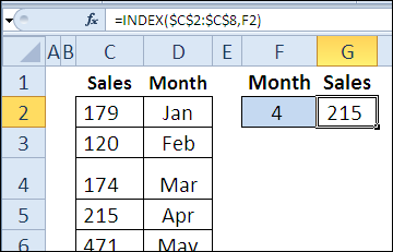
Example 1: Find the amount of sales for the selected month

Enter the line number, and the function INDEX (INDEX) will return the amount of sales from this row. Here is the number of the month 4, so the result will be the sum of sales for April (Apr).

=INDEX($C$2:$C$8,F2)

=ИНДЕКС($C$2:$C$8;F2)

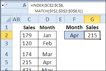
To make this formula more flexible, you can use the function MATCH (MATCH) to determine the row number by month, which can be selected from the drop-down list.

=INDEX($C$2:$C$8,MATCH($F$2,$D$2:$D$8,0))

=ИНДЕКС($C$2:$C$8;ПОИСКПОЗ($F$2;$D$2:$D$8;0))

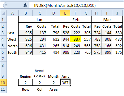
Example 2: Getting a reference to a specific row, column, or area

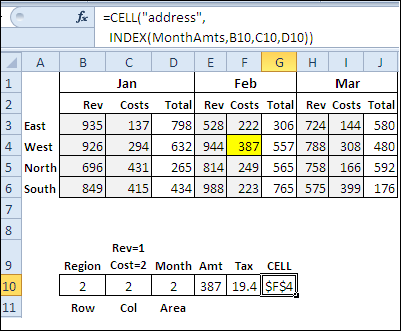
In this example, the named range MonthAmts consists of 3 non-adjacent ranges. Range MonthAmts has 3 areas – one for each month – and each area has 4 rows and 2 columns. Here is the formula for the name MonthAmts:

='Ex02'!$B$3:$C$6,'Ex02'!$E$3:$F$6,'Ex02'!$H$3:$I$6

='Ex02'!$B$3:$C$6;'Ex02'!$E$3:$F$6;'Ex02'!$H$3:$I$6

Using functions INDEX (INDEX) You can return the cost (Cost) or the amount of revenue (Rev) for a specific region and month.

=INDEX(MonthAmts,B10,C10,D10)

=ИНДЕКС(MonthAmts;B10;C10;D10)

With function result INDEX (INDEX) you can perform a multiplication operation, as when calculating the tax (Tax) in cell F10:

=0.05*INDEX(MonthAmts,B10,C10,D10)

=0,05*ИНДЕКС(MonthAmts;B10;C10;D10)

or it can return a function reference CELL (CELL) to show the address of the result in cell G10.

=CELL("address",INDEX(MonthAmts,B10,C10,D10))

=ЯЧЕЙКА("адрес";ИНДЕКС(MonthAmts;B10;C10;D10))

Example 3: Creating a Dynamic Range Based on a Count

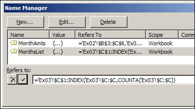
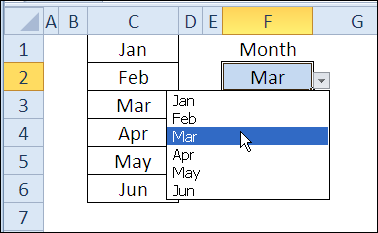
You can use the function INDEX (INDEX) to create a dynamic range. This example created a named range MonthList with this formula:

='Ex03'!$C$1:INDEX('Ex03'!$C:$C,COUNTA('Ex03'!$C:$C))

='Ex03'!$C$1:ИНДЕКС('Ex03'!$C:$C;СЧЁТЗ('Ex03'!$C:$C))

If you add another month to the list in column C, it will automatically appear in the drop-down list in cell F2, which uses MonthListas a data source.

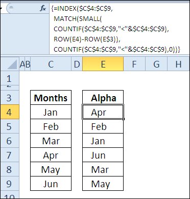
Example 4: Sort a column of text data alphabetically

In the final example, the function INDEX (INDEX) works in conjunction with several other functions to return a list of months sorted alphabetically. Function COUNTIF (COUNTIF) counts how many months come before each specific month in the list (an array is created). SMALL (SMALL) returns the nth smallest value in the created array, and MATCH (MATCH) returns the row number of the desired month based on this value.

This formula must be entered in cell E4 as an array formula by pressing Ctrl + Shift + Enter. And then copied from the rest of the cells in the range E4:E9.

=INDEX($C$4:$C$9,MATCH(SMALL(COUNTIF($C$4:$C$9,"<"&$C$4:$C$9),
ROW(E4)-ROW(E$3)),COUNTIF($C$4:$C$9,"<"&$C$4:$C$9),0))

=ИНДЕКС($C$4:$C$9;ПОИСКПОЗ(НАИМЕНЬШИЙ(СЧЁТЕСЛИ($C$4:$C$9;"<"&$C$4:$C$9);
СТРОКА(E4)-СТРОКА(E$3));СЧЁТЕСЛИ($C$4:$C$9;"<"&$C$4:$C$9);0))