


Contents
Many Excel users are well aware of the function SUM. It allows you to sum several values or a whole range at once. But few people know that there is a function that allows you to significantly expand its functionality. It is, as you can guess, the function SUMMESLI.
Understanding the SUMIF function
As the name implies, this function sums up the values that meet a certain condition. It allows you to replace a complex formula with a single function.
Syntax of the SUMIF function
This function has the following arguments:
- Search range. This is the set of cells that will be checked against the conditions.
- Condition. This argument is enclosed in quotation marks. This is directly the criterion under which the cells will be summed up.
- Summation range. If you want to check certain cells against the specified criteria, use this argument. It’s optional. If it is not specified, the summation will be carried out in the search range.
How the SUMIF function works in Excel
It is very easy to demonstrate how this function works with such a simple example. Suppose we have a table that lists the names of employees, their gender, position and salaries. If we need to understand how much money we need to pay them in general, then the function is used SUM with a single argument – the range of salaries.
But what if you need to calculate the total amount of salaries that are paid to sellers? In this case, you need to use a more advanced function SUMMESLI.
Let’s describe the arguments.
- The column with positions is used as the search range. Of course, the column header is not included in it.
- The condition used is the seller. Don’t forget to enclose this argument in quotation marks.
- In our case, wages are used as the summation range. Accordingly, the value of this argument is F2:F14.
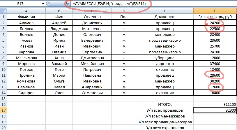

1
The resulting result is 92900. Agree that this is much more convenient than manually analyzing the list of professions, checking them for compliance with a certain condition, and then also summing up these values. Especially if the table is large.
In the same way, the salary of all other employees is calculated.
SUMIF function in Excel with multiple conditions
This function has a modification that allows you to add multiple conditions to the formula. It is enough to add two letters MN to the end of its name. Get SUMIF. If there is more than one criteria, then you need to use this function.
Syntax
You can use an unlimited number of arguments, but you must specify 5 as a minimum.
- Summation range. This is the main argument here, which must be specified. The value is the same – an indication of specific cells that need to be summed.
- The range of the first condition. Argument equivalent to the search range in the SUMIF function. Only in this case specifies the range of the first criterion.
- First condition.
- The range of the second condition. Arguments similar to the range of the first condition.
- Second condition.
Further logic is the same. The search range is specified, and then the criterion itself. Thus, as the number of criteria increases, the number of arguments increases in an arithmetic progression, where the step is two: 5,7,9,11 and so on.
Application example
Let’s say we need to calculate the amount of salary per month for all female salespeople who meet two criteria:
- They are women.
- They are sellers.
Therefore, to implement this task, you need to use the SUMIFS function.
In our case, the arguments will be as follows:
- As the summation range, we leave the same range as in the previous example (since it contains salaries).
- Condition range 1 – the profession of the worker.
- Condition 1 – the seller.
- Range of conditions 2 – gender of the worker.
- Condition 2 – female
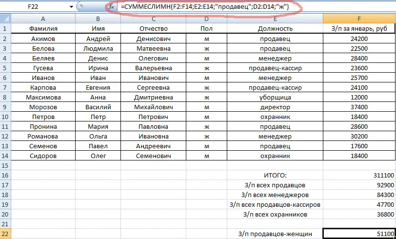

2
This is how it works in practice. The total amount of money that was received amounted to 51100 rubles.
SUMIF function with dynamic condition
Both variations of the SUMIF function, both with one criterion and with several, can adapt to their change. Simply put, if you change the values in the specified range, the amounts will be automatically adjusted. Let’s say that in the payroll it was discovered that one sales employee was not taken into account. We have the opportunity to correct this situation by adding an additional line and entering the appropriate data.
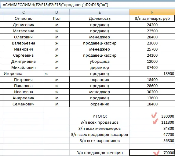
It immediately becomes clear that both ranges, both conditions and summation, have been increased by one line.
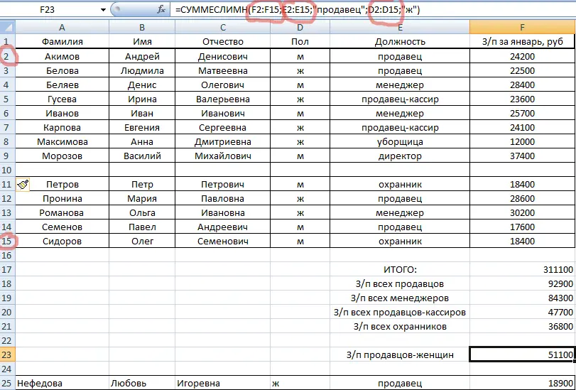
After information about the employee was added to the general list, the formula automatically recalculated the values based on the new data. The functions responded to the addition of another saleswoman to the list.
This mechanism extends not only to added lines, but also to deleted ones. For example, you can fire an employee, and the program will automatically recalculate the required values. You can also change the values. For example, you can make a new one based on an old report, just replace the name of the month and put updated salaries, after which the program will automatically change the converted template to the current situation.
Examples of using the SUMIF function
In practice, everything is simple. But in reality, there may be some difficulties associated with the peculiarities of the tasks that need to be solved. Here are a few examples to better understand how you can use the function SUMMESLI. Let’s start with the simplest tasks and finish with the more complex ones.
The use of this function does not differ in different versions of the Microsoft Office suite. Also, if you study in detail the features of using this function, it will be much easier to understand how formulas work. COUNTIF, COUNTIFS and others like that.
Sum by multiple conditions
We have already understood that the standard function SUMMESLI works with only one condition, while it is often necessary to define a data set that simultaneously meets several conditions at once. To do this, you can use some tricks or apply other functions.
Suppose we have a table with orders. And our task is to determine the total number of orders for different types of chocolate.
The first method is using two functions SUMMESLI.

We have used the formula =СУММЕСЛИ($C$2:$C$21;»*»&H3&»*»;$E$2:$E$21)+СУММЕСЛИ($C$2:$C$21;»*»&H4&»*»;$E$2:$E$21)
In this case, we tried to determine the total number of orders for goods of each type, after which the addition operation was performed. Everything is simple.
But, of course, this method has a drawback – low universality. Therefore, we need to consider the second option, which involves the use of functions SUM и SUMMESLI with array arguments.
This method allows you to process a large amount of data and criteria at once. In this case, you need to specify an entire array of conditions as an argument at once. Let’s take a closer look at this method.

You can start by describing all the conditions, successively separated by a semicolon, after which the resulting result should be enclosed in curly brackets. Such an argument is called an array argument, and the resulting formula will look like this.
=SUMIF($C$2:$C$21;{“*black*”;”*milk*”};$E$2:$E$21)
Since a whole array of conditions is used here, the resulting value will also be an array, which includes two values.
The last step is to use the SUM function, which can perform an addition operation on the information inside the array. Get this formula.
=SUM(SUMIF($C$2:$C$21,{“*black*”;”*milky*”},$E$2:$E$21))
As you can see, the calculation results are the same in both cases.
Another option for using multiple criteria is a combination of functions. SUMMESLI и SUMPRODUCT. This makes it possible to list conditions in a separate part of the range.
The formula will be like this.
=СУММПРОИЗВ(СУММЕСЛИ(C2:C21;H3:H4;E2:E21))
As you can see from this formula, the criteria are written in cells with addresses H3 and H4. But it is also possible to use an array of criteria, as in the previous example.
=SUMPRODUCT(SUMIF(C2:C21,{“*black*”,”*milky*”},E2:E21))

The returned result will still be the same, it’s just that some formulas are more convenient to use in some situations, and others in others.
It is important to consider that all the methods described above are necessary to specify one of the conditions. That is, the logical OR operation is used. To sum values that match more than one condition at the same time, use the SUMIFS function.
Sum of values corresponding to blank or non-blank cells
There are situations when, as a criterion, you need to specify all the filled cells, where at least something is written, regardless of the type. Let’s take another example of how this function can be used. Imagine that we have a table in which we need to understand how many orders have not been completed, and how many have already been processed.

To account for non-blank cells, the asterisk (*) symbol is used as a criterion. In our case, the formula will be as follows.
=СУММЕСЛИ(F2:F21;»*»;E2:E21)
A similar result can be obtained if you use such a character set – .
=СУММЕСЛИ(F2:F21;»»;E2:E21)
To search for empty cells, you need to write paired single quotes in the argument with the criterion, which are written if the value of the condition is written in the cell, and the formula simply contains a reference to it.
If it is necessary to summarize only empty cells that are contained in the formula itself, then you can simply specify double quotes as the second argument.
=СУММЕСЛИ(F2:F21;»»;E2:E21)
Exact date, date range
If you want to sum up the numbers that relate to a specific date, then you need to write it down as a condition.
It is important to consider that the format must match the one indicated in the table.
Here you can also use a reference to the argument or enter it directly into the formula.

Now it remains to calculate the sales results for today. This can be done either by specifying the date in the second argument (or cell), or by writing the function TODAY().
=SUMIF(A2:A21,TODAY(),E2:E21)
If used in an argument TODAY()-1, then “yesterday” will be used as the criterion.
Wildcards for Partial Match
Sometimes you need to look not for the whole phrase, but for part of it. To do this, there are symbols that replace a certain part of the argument.
- ? – replacement of any character.
- * – replace any number of characters.
For example, three question marks matches any word that consists of three letters.
To use as an argument a value containing the characters themselves ? and *, then you need to write a ~ sign in front of them. Then they will be considered plain text, not a template.

Criteria for text
Often it is necessary to select meanings for certain words. In this case, you need to use the text as an argument. It can be either directly written in the formula, or be in a separate cell with a link to it.
=СУММЕСЛИ(F2:F21;I2;E2:Е21)
Do not forget to enclose all text values in quotation marks.
Sum if “greater than”, “less than”, “equal to”
In this case, you must write the appropriate logical operator before the argument enclosed in quotes. For example, yes.
=SUMIF(D2:D21,”
In this example, all orders that are less than 144 will be summed up. There is no point in specifying “equals” directly, because such a logical operator is used by default.

Why might the SUMIF function not work?
There are several common mistakes that the function SUMMESLI stops working.
- Ranges must be specified as range references, not an array. This error is quite rare, but it’s possible because many beginners don’t fully understand the difference between a range and an array.
- If values from other worksheets or workbooks that are closed at the time the formula is used are summed up.
- The range of data and search differ in size.
Thus, there are quite a few situations where the formula does not work. Generally, SUMMESLI – This is a very simple function, which even a beginner can master.