


Contents
A fairly common difficulty that Excel users face when trying to copy numeric information or import files is when the numeric format becomes text. Because of this, the formulas lose their working capacity, which makes any calculations unrealistic. What can be done to quickly fix this problem?
How to convert text to number in Excel?
In general, the classic method is the use of macros. But there are some ways that do not involve programming.
Green corner-indicator
The fact that the number format has been converted to text is indicated by the appearance of a kind of indicator corner. Its appearance is a kind of luck, because it is enough to select everything, click on the pop-up icon and click on “Convert to Number”.
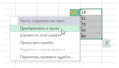
All values written as text but containing numbers are converted to a number format. It may also happen that there are no corners at all. Then you need to make sure that they are not disabled in the program settings. They are on the way File – Options – Formulas – Numbers, formatted as text or preceded by an apostrophe.
Re-entry
If there are a small number of cells whose format was incorrectly converted, then you can enter the data again than change it manually. To do this, click on the cell of interest and then – the F2 key. After that, a standard input field appears, where you need to retype the value, and then press Enter.
You can also double-click on a cell to achieve the same goal. Of course, this method will not work well if there are too many cells in the document.
Text to number formula
If you create another column next to the one where the numbers are in the wrong format and write one simple formula, it will automatically be converted to a numeric one. It is shown in the screenshot.
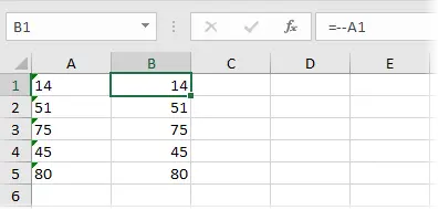
Here, the double minus replaces the operation of multiplying by -1 twice. Why is this being done? The fact is that minus by minus gives a positive result, so the result will not change. but since Excel performed an arithmetic operation, the value cannot be anything other than a numeric value.
It is logical that you can use any such operation, after which there is no change in value. For example, add and subtract one or divide by 1. The result will be the same.
Paste special
This is a very old method that was used in the first versions of Excel (because the green indicator was added only in the 2003 version). Our actions are as follows:
- Enter a unit in any cell that does not contain any values.
- Copy it.
- Select cells with numbers written in text format and change it to numeric. At this stage, nothing will change, so we perform the next stage.
- Call the menu and use Paste Special or Ctrl + Alt + V.
- A window will open in which we are interested in the radio button “values”, “multiply”.


3
In fact, this operation performs similar actions to the previous method. The only difference is that not formulas are used, but the clipboard.
Text in Columns tool
There may sometimes be a more complex situation where the numbers contained a delimiter that might still be in the wrong format. In this case, another method must be used. You need to select the cells that need to be modified and click on the “Text by columns” button, which can be found on the “Data” tab.
It was originally created for a different purpose, namely to split text that was not joined correctly into multiple columns. But in this situation, we use it for other purposes.
A wizard will appear in which the configuration is carried out in three steps. We need to skip two of them. To do this, just double-click “Next”. After that, our window will appear in which you can specify the separators. Before that, you need to click on the “Advanced” button.
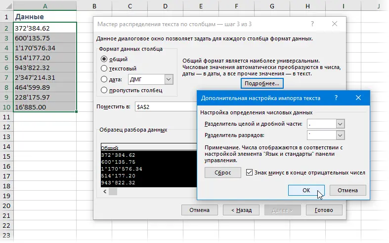
It remains only to click on “Finish”, as the text value will immediately turn into a full number.
Text to Number Macro
If you often need to perform such operations, then it is recommended to make this process automatic. To do this, there are special executable modules – macros. To open the editor, there is a combination of Alt + F11. It can also be accessed through the Developer tab. There you will find the “Visual Basic” button, which you need to click.
Our next task is to insert a new module. To do this, you need to open the menu Insert – Module. Next, you need to copy this code fragment and paste it into the editor in the standard way (Ctrl + C and Ctrl + V).
Sub Convert_Text_to_Numbers()
Selection.NumberFormat = «General»
Selection.Value = Selection.Value
End Sub
To perform any actions with a range, it must first be selected. After that, you need to run the macro. This is done through the “Developer – Macros” tab. A list of routines that can be executed in the document will appear. We need to select the one that we need and click on “Run”. Then the program will do everything for you.
How to define numbers written in Excel as text?
As it became clear from the above, Excel displays possible format problems in two ways. The first is the green triangle. The second is a yellow exclamation mark that appears when a cell with the previous designation is selected. To be more specific about this problem, you need to hover over the pop-up sign.
If a numeric cell is formatted as text, Excel warns about this with the appropriate inscription.
We know that in some cases the triangle does not appear (or the Excel version is too old). Therefore, to determine what format the cell is, you can use the analysis of other visual features:
- Numbers are normally on the right side, while values in text format are on the opposite side.
- If you select a data set with numerical values, at the bottom it will be possible to immediately calculate the sum, average value and a number of other parameters.
How to use the error indicator?
Users often ask this question, but this method has already been described above. If an indicator appears indicating an error, you can convert the format in just one click. To do this, select the range and click on “Convert to Number”.
Removing non-printing characters
If you copy information from other sources, then often a lot of garbage is transferred along with useful information, which would be nice to get rid of. Some of this garbage is non-printable characters. Because of them, a numeric value can be perceived as a set of characters.
To get rid of this problem, you can use the formula =VALUE(TRIMSPACES(CORRECT(A2)))
The way this formula works is very simple. Using the function PRINT you can get rid of non-printable characters. In turn, TRIM removes invisible spaces from a cell. A function ZNAChEN makes text characters numeric.
Extract number from text
This feature will be useful if you need to extract a number from a string. To do this, it must be used in combination with the functions RIGHT, LEFT, PSTR.
So, to get the last 3 characters from cell A2, and return the result as a number, you need to apply this formula.
=SIGNIFICANT(TRUESYMPHO(A2))
If you don’t use the function RIGHT inside a function ZNAChEN, then the result will be in character format, which makes it difficult to perform any computational operations with the resulting numbers.
This method can be used in situations where a person is aware of how many characters to extract from the text, as well as where they are located.