This is a simple but interesting trick that allows you to substitute data from small tables without using cells at all. Its essence is that you can “sew” an array of substitution values directly into the formula. Let’s look at several ways to do this.
SELECT function
If you need to substitute data from a one-dimensional array by number, then you can use the INDEX function or its simpler and more suitable, in this case, analogue – the function SELECTION (CHOOSE). It outputs an array element by its ordinal number. So, for example, if we need to display the name of the day of the week by its number, then we can use this construction

This is a simple example to start with to get the idea that a lookup table can be wired right into a formula. Now let’s look at a more complicated, but prettier example.
Array of constants in formula
Suppose we have a list of cities, where using the function VPR (VLOOKUP) the values of the salary coefficients from the second column of the yellow table on the right are substituted:
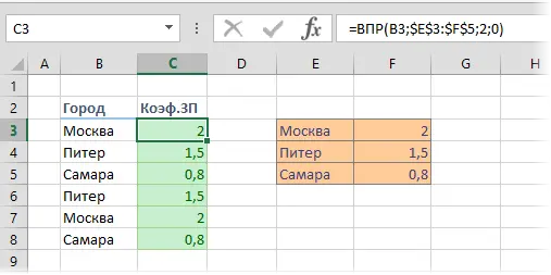
The trick is that you can replace the reference to a range with table $E$3:$F$5 array of constants directly in the formula, and the right table will no longer be needed. In order not to enter data manually, you can go for a little trick.
Select any empty cell. Enter the equal sign from the keyboard and select the range with the table – its address should be displayed in the formula bar:
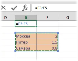
Select with the mouse the link E3:F5 in the formula bar and press the key F9 – the link will turn into an array of constants:
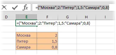
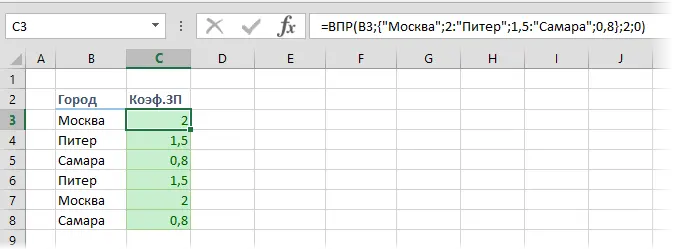
It remains to copy the resulting array and paste it into our formula with VLOOKUP, and delete the table itself as unnecessary:
Named array of constants
Developing the idea of the previous method, you can try another option – to do named array of constants in RAM, which is then used in the formula. To do this, click on the tab formula (Formulas) button Name Manager (NameManager)… Then press the button Create, think up and enter a name (let it be, for example, Cities) and in the field Range (Reference) paste the array of constants copied in the previous method:
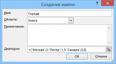
Press OK and close Name Manager. Now the added name can be safely used on any sheet of the book in any formula – for example, in our VLOOKUP function:
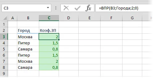
Compact, beautiful and, in a sense, even protects from playful hands of non-professionals 🙂
- How to use the VLOOKUP function to lookup data from one table to another
- How to use approximate search with the VLOOKUP function
- Calculations without formulas


