How to create your own data format in Excel

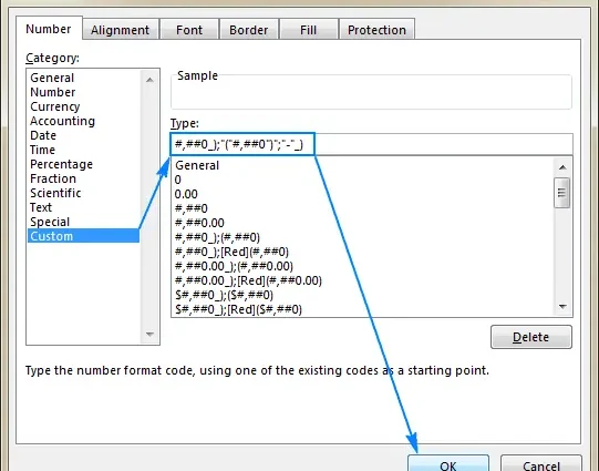
The data format in Microsoft Office Excel is the type of display of characters in the cells of a table array. The program itself has many standard formatting options. However, sometimes you need to create a custom format. How to do this will be discussed in this article.

How to change cell format in Excel

Before you start creating your own format, you need to familiarize yourself with the principles of changing it. You can change one type of information display in table cells to another according to the following scheme:

1. Click the left mouse button on the required cell with data to select it.
2. Right-click anywhere in the selected area.
3. In the context menu, click on the line “Format Cells …”.
4. In the window that opens, go to the “Number” section and in the “Number formats” block, select one of the appropriate options by clicking on it twice with LMB.

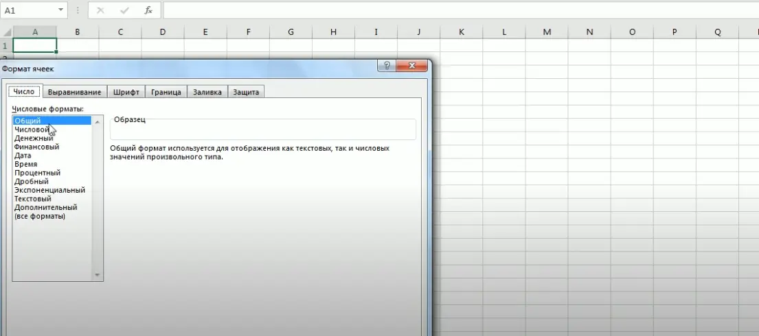
5. Click “OK” at the bottom of the window to apply the action.

Pay attention! After changing the format, the numbers in the table cells will be displayed differently.

How to create your own format in Excel

The principle of adding a custom data format in the program under consideration can be divided into several stages:

1. Select an empty cell of the worksheet and, according to the above scheme, go to the “Format Cells …” window.
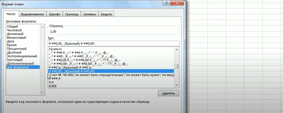
2. To create your own format, you need to write a certain set of codes in a line. To do this, select the “All formats” item and in the next window in the “Type” field enter your own format, knowing its encoding in Excel. In this case, each section of the code is separated from the previous one by a semicolon.

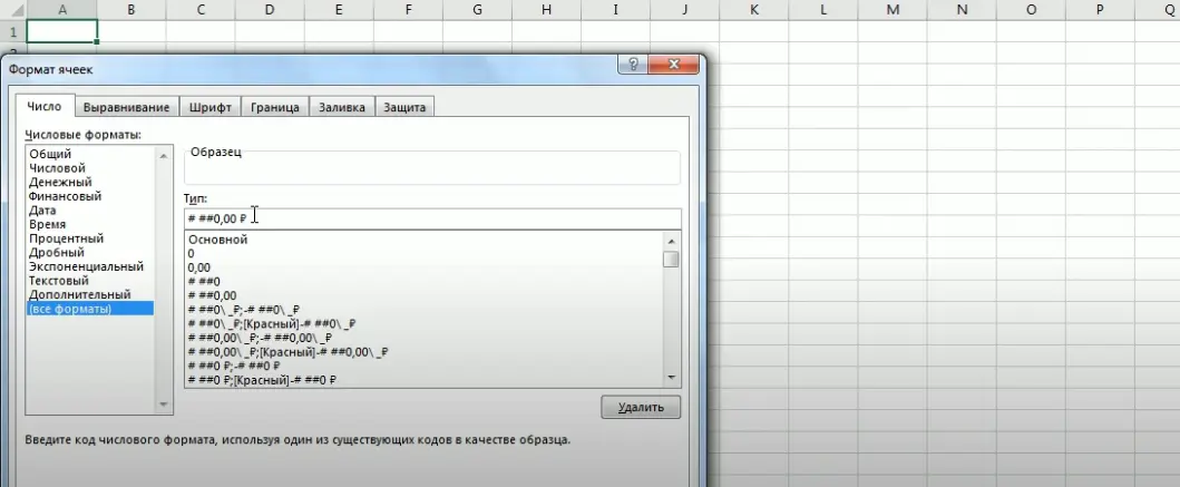
3. Check how Microsoft Office Excel encodes a particular format. To do this, select any encoding option from the list available in the window and click on “OK”.
4. Now, in the selected cell, you must enter any number, for example, one.

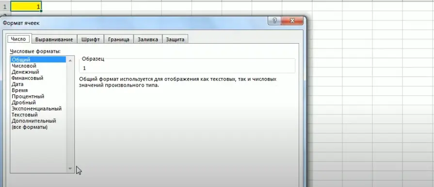
5. By analogy, enter the cell format menu and click on the word “Numeric” in the list of presented values. Now, if you go to the “All formats” section again, then the selected “Numeric” formatting will already be displayed as an encoding consisting of two sections: a separator and a semicolon. Sections will be shown in the “Type” field, with the first of them characterizing a positive number, and the second one is used for negative values.

6. At this stage, when the user has already figured out the principle of coding, he can start creating his own format. For this purpose, he first needs to close the Format Cells menu.
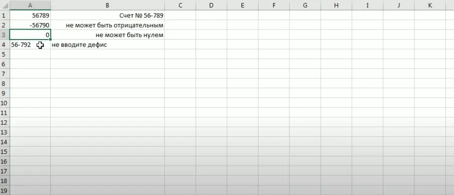
7. On the Excel worksheet, create the initial table array shown in the image below. This table is considered as an example; in practice, you can create any other plate.

8. Insert an additional column between the original two.

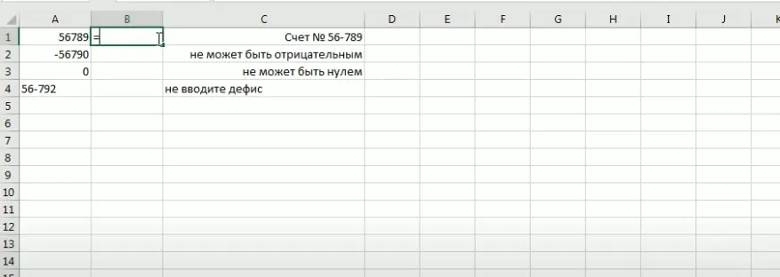
Important! To create an empty column, you need to right-click on any column of the table array and click on the “Insert” line in the context window.

9. In the column created manually from the PC keyboard, you must enter the data from the first column of the table.

10. Select the added column and right-click on it. Go to the cell format window according to the scheme discussed above.
11. Go to the “All formats” tab. Initially, the word “Main” will be written in the “Type” line. It will need to be replaced with its own value.
12. The first place in the format code must be a positive value. Here we prescribe the word “”Not negative””. All expressions must be enclosed in quotes.
13. After the first value, put a semicolon and write “”not zero””.
14. Once again we put a semicolon and write the combination “” without a hyphen “”.
15. At the very beginning of the line, you will also need to write “Account No.”, and then set your own format, for example, “00-000 ″”.

16. Save the changes by clicking on “OK” at the bottom of the window and expand the column added earlier to see specific values ​​​​instead of the characters “####”. Phrases from the created format will be written there.

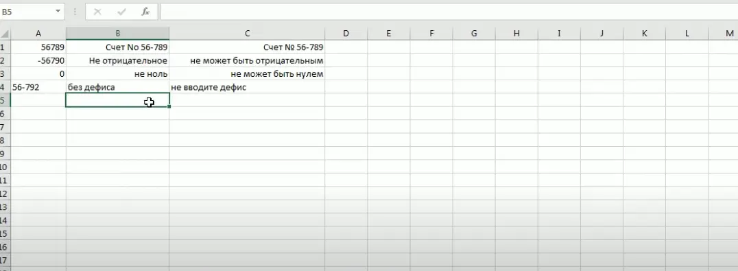
Additional Information! If the information in the cells is not displayed, then the user made a mistake when creating their own format. To correct the situation, you will need to go back to the tabular array element formatting settings window and check the correctness of the entered data.

How to remove unwanted data format in Microsoft Office Excel

If a person does not want to use one or another standard program format, then he can uninstall it from the list of available values. To cope with the task in the shortest possible time, you can use the following algorithm:

1. Click with the left mouse button on any cell of the table array. You can simply click on an empty worksheet element.
2. In the context type box, click on the “Format Cells” line.
3. Move to the “Number” section in the top toolbar of the menu that opens.
4. Select the appropriate number format from the list of the boxes on the left and select it by clicking LMB.
5. Click on the “Delete” button, which is located in the lower right corner of the “Format Cells” window.
6. Agree with the system warning and click OK to close the window. The selected standard or custom format should be deleted from MS Excel without the possibility of recovery in the future.

Conclusion

Thus, adding custom formats to Microsoft Office Excel is a simple procedure that you can handle on your own. To save time and simplify the task, it is recommended to use the above instructions.