How to create a pivot table in Excel. 2 Ways to Create a PivotTable in Excel

A filter-driven table report helps organize information in large databases. Let’s find out how to create such a table based on information from an Excel document and edit its form and content.

How to Create a PivotTable in Excel

Before compiling a summary plate, it is necessary to check whether its components meet several criteria. If you do not pay attention to this, problems may arise in the future. The conditions are:

• above each column there is a header with a heading;
• each cell in the table is filled;
• cell formats are set (for example, only the “Date” format for dates);
• one cell contains data of only one format;
• you need to split the merged cells.

Let’s consider two methods of creating a tabular report.

The classic way to create a pivot table

To test this method, we will use a tablet with data on sales of sporting goods. You need to set the goal of creating a table in order to clearly present the result. Let’s use the data to figure out how many women’s tennis shoes were sold in the store. The amount should appear on the line next to the title, even if the sales are spread across multiple lines in the source.

It is possible to simplify the updating of the pivot table by connecting dynamic changes. When new information is added to the initial table, the calculation result will change. This is an optional step.

1. Click on one of the source cells and open the Home tab at the top of the screen. You need to find the “Styles” section, and in it – the “Format as table” function. Choose your favorite style.

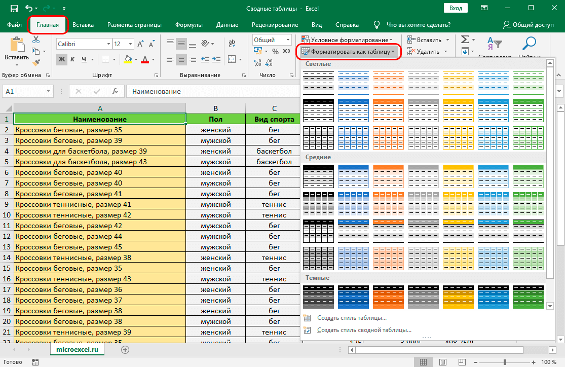
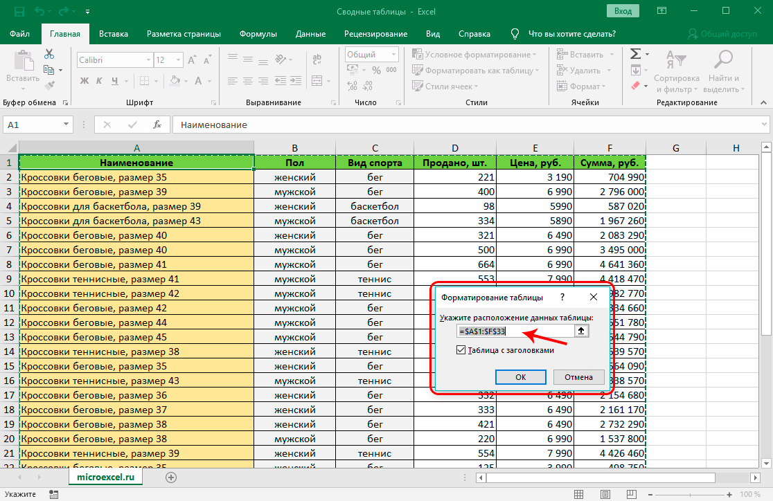
2. A window will appear on the screen where you want to add a range of data. Usually the line is already filled in, it remains to check the coordinates, check the box “Table with headers” and click “OK”.

The Table Design tab appears on the toolbar. It will appear at the top of the screen every time you select cells in a formatted table. The program gives the table a name, you can always change it. Let’s move on to the main stage – drawing up a tabular report:

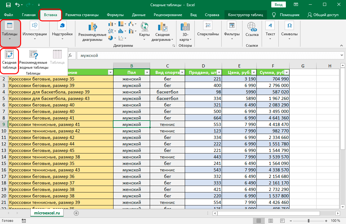
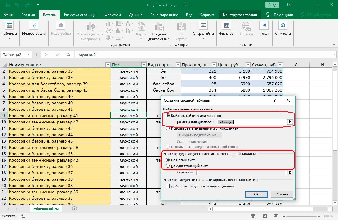
1. You need to open the “Insert” tab, click on the “Pivot Table” item on the left side of the screen.

2. A window for creating a pivot table will appear on the screen. Select the data range from which the report will be generated. First, the name of the first plate will appear in the line – if necessary, you can select other cells or specify the name of another table from the same document.
3. Let’s choose the place where the pivot table will be placed. It can be placed on the same sheet or on a new one in the same document as the initial data.
4. After filling in all the fields, click “OK”.

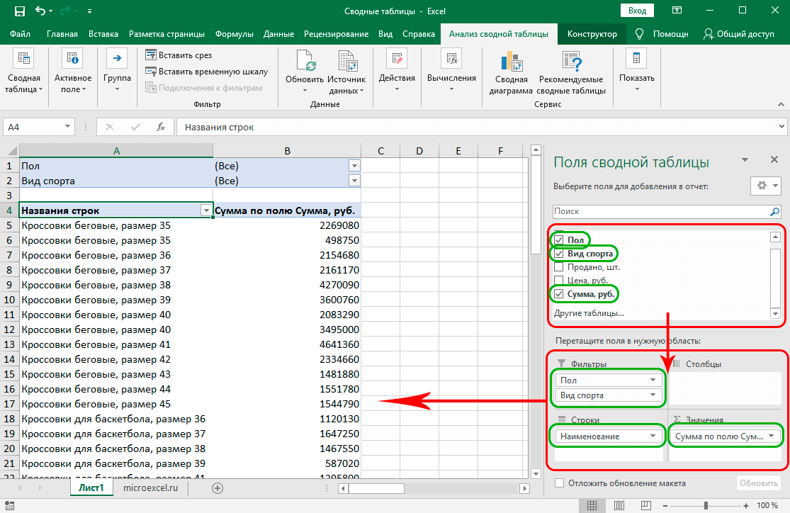
5. A window for generating a table will open. It contains a list of fields and settings areas. Select the required fields at the top of the window. After that, drag them to the desired areas.

In a given situation, several fields are needed. “Gender” and “Sport” fall into the “Filters” category, “Name” – into the “Lines” area, “Amount” is moved to “Value”. The Columns section remains empty.

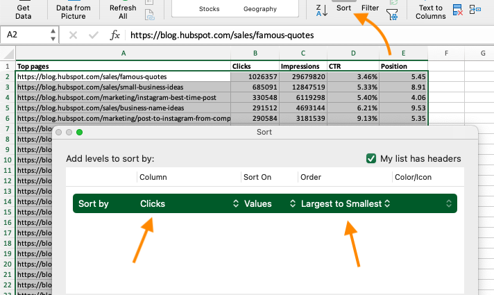
When the table is formed, you need to apply the selected filters. Let’s break this down step by step. It is worth remembering the condition: you need to determine the sales of women’s tennis shoes.

1. Open the “Gender” section in the table and select “Female”, then click “OK”.

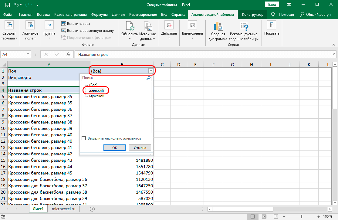
2. Apply the filter to the sport – according to the condition, you must check the box “Tennis” and click “OK”.

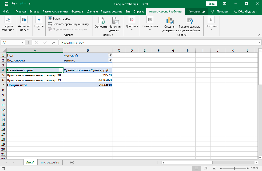
Result: Only the requested data is presented on the sheet. Information about the amount in several lines with the same name is summarized.

Using the PivotTable Wizard

You can create a report using a special tool – PivotTable Wizard. The function is not in quick access by default, so let’s add it there first.

1. Open the “File” tab, its “Options” section. We find the item “Quick Access Toolbar”, in the list that appears, select the item “PivotTable and PivotChart Wizard”. The “Add” button will become active, you need to click on it, and then click “OK”.

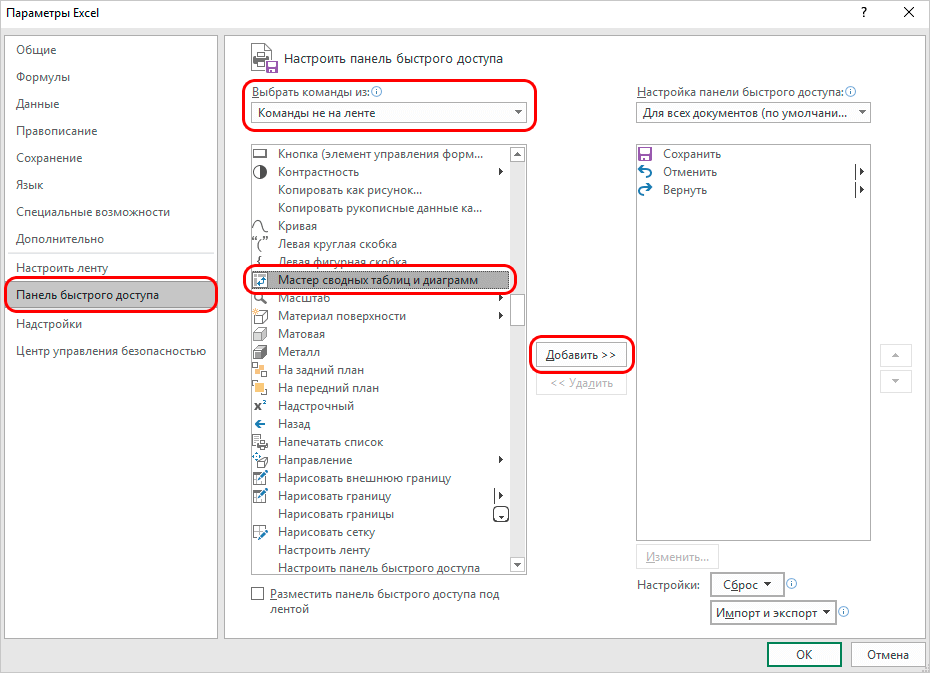
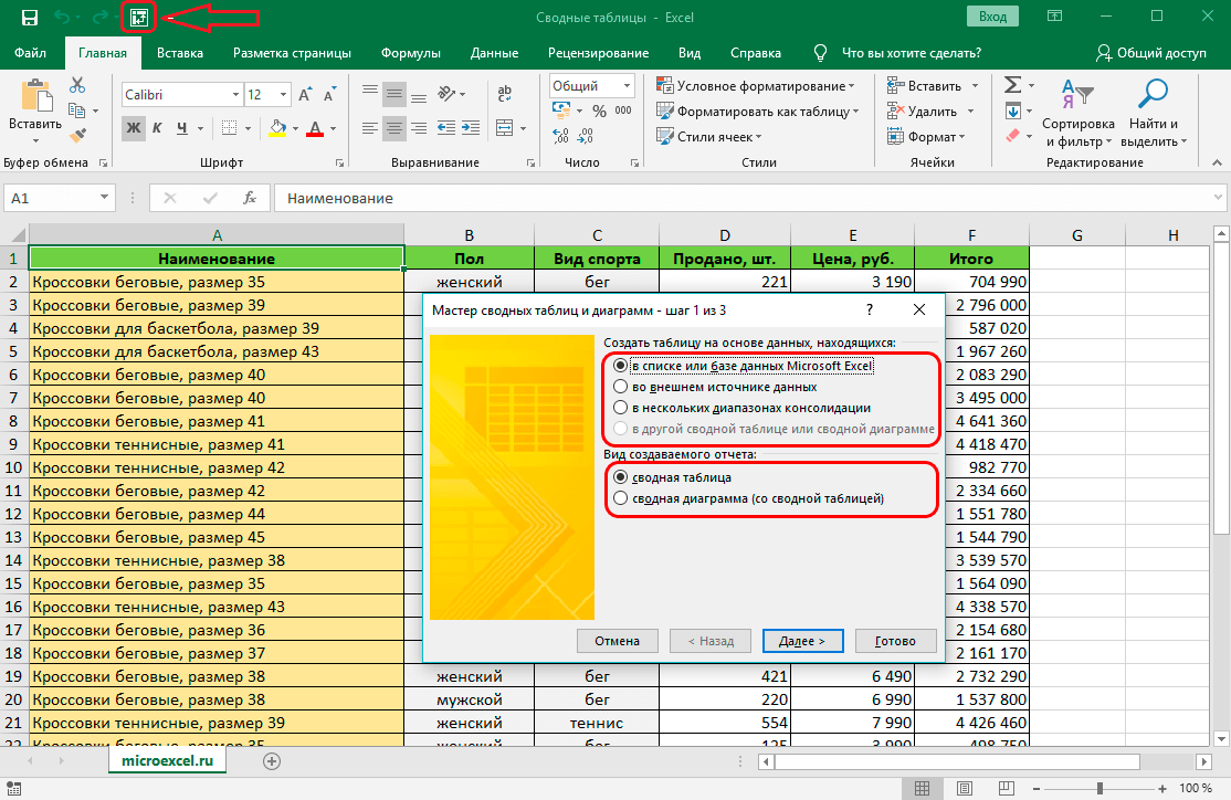
2. We start working with the PivotTable Wizard by clicking on the square icon that appears in the upper left corner of the screen.
3. The Wizard window will appear. It is necessary to define the source of information and the type of report. In the first case, select the first item – a list or database, in the second – a pivot table.

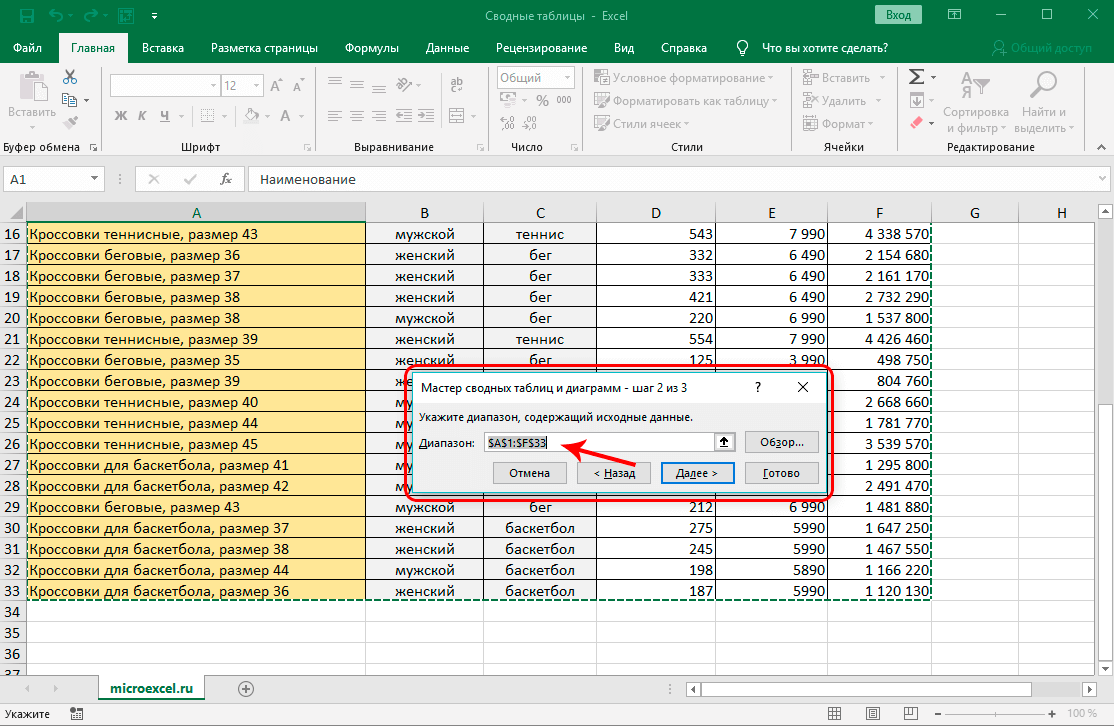
4. The second step of working with the Wizard is defining the data range. The program automatically selects the range, so you need to check if it is correct. If the data is selected incorrectly, select the cells manually. After setting the range, click “Next”.

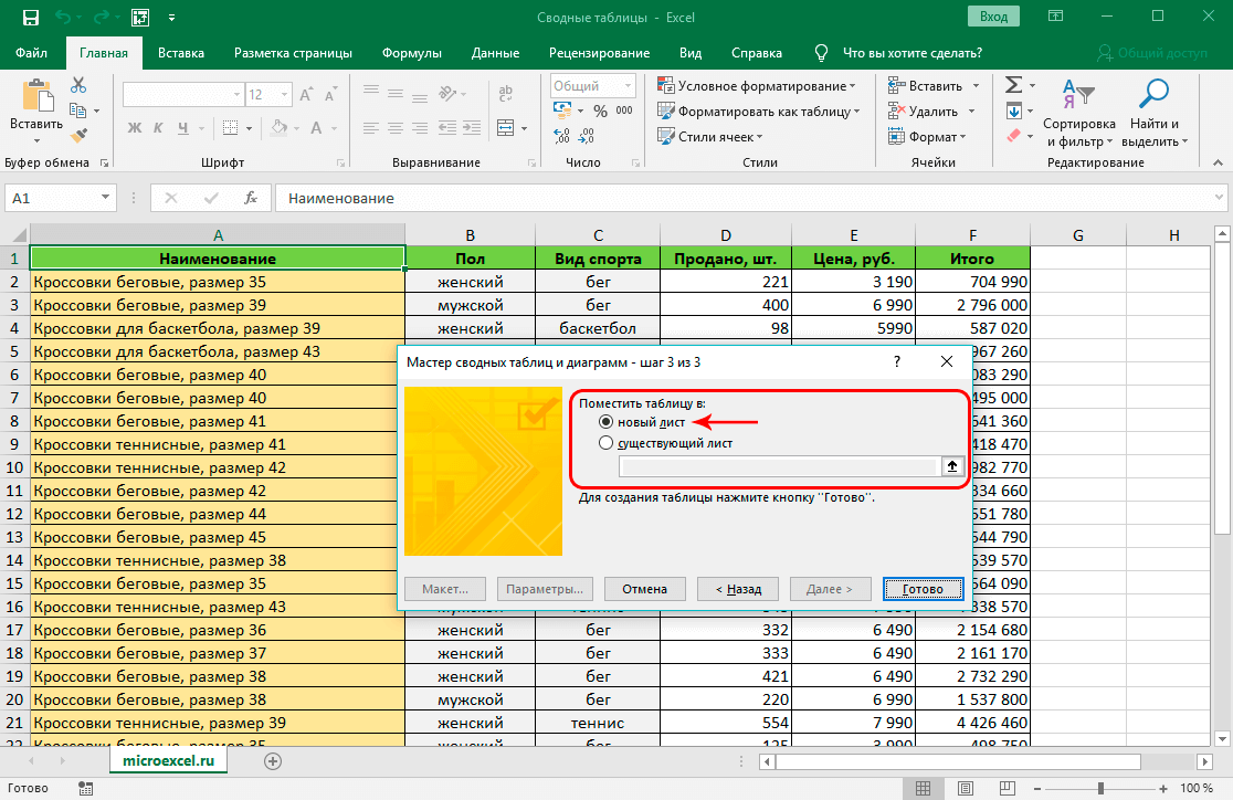
5. We determine where we are going to place the summary plate. If you select “Existing sheet”, specify a specific sheet from the document.

6. We fill in the form of the summary plate according to the rules of the classical method and set the filters.

How to make a pivot table from multiple tables

Often, data that is important for a report is located in different tables and needs to be combined. Let’s use the PivotTable Wizard and combine several databases into one. Imagine that there are two tables with data on the availability of goods in a warehouse. You need to use Excel tools to combine them into one database.

1. Select a cell and open the PivotTable and PivotChart Wizard. If it is already on the quick access panel, you need to click on the corresponding icon. To learn how to add a tool to a panel, see Using the PivotTable Wizard.
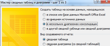
2. The data is in two sources, so we select the item “In several consolidation ranges”. You also need to select the type of report – “pivot table”.

3. In the next step, select the item “Create data fields” and click “Next”.
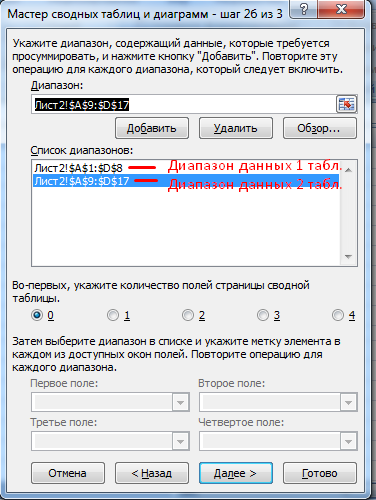
4. A window with a list of ranges will appear. You can add multiple tables there. We select the first table with the mouse and click “Add”, we do the same with the second table.

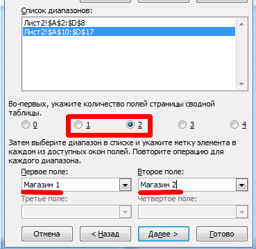
5. We select the ranges in turn and give them names as fields in the pivot table. You also need to specify the number of fields.

6. The last step is to choose a location for the report. It will be more convenient to use a new sheet, so the new table will not disturb the location of other information in the document.

How to make a pivot table in Excel from multiple sheets

Data on the activities of the company sometimes appear on different sheets in one document. Let’s use the PivotTable Wizard again to get a summary report.

1. Open the PivotTable and PivotChart Wizard. In the window of the first step, you need to select the data source “in different consolidation ranges” and the type “pivot table”.
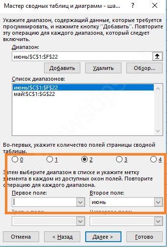
2. In the second step, select the “Create page fields” item. The range selection window will open. First, select the cells with information on the first sheet and click the “Add” button. Next, you need to switch to the next sheet with data, select them and click the “Add” button. After entering all the cells in the list, select the number of fields and their order. If the information is added correctly, you can proceed to the next step by clicking the “Next” button.

3. We place the plate on a new sheet or on one of the existing sheets and click “Finish”.

Important points to consider when creating pivot tables

There are several features that should be taken into account when working with reports in the form of tables:

• check whether the names and other information are spelled out correctly in each line, otherwise the report will be compiled taking into account typos – several lines will be created for one name;
• it is necessary to fill the entire header if the table is not converted to dynamic in order to avoid errors;
• if the report data does not change automatically (that is, it is not dynamic), you need to update the information after making changes to the sources.

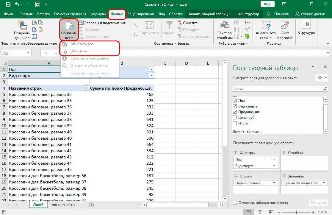
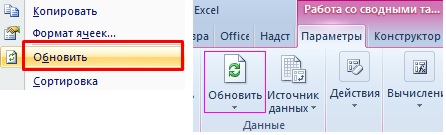
Important! You can update the summary table through the “Data” tab. To do this, select a cell in the table and find the “Update All” function on the tab.

Benefits of pivot tables

PivotTable reports have significant advantages over other types of reports in Excel. Let’s consider each of them:

1. The table is compiled on almost any amount of data.
2. You can edit the report view through the format menu – the built-in library contains many color themes for tables.
3. It is possible to combine data into broader groups, for example, several dates are combined into quarters.
4. Based on the results of the report, you can carry out calculations using Excel tools, this will not affect the data sources.
5. The information in a PivotTable can form the basis for a graph or other visual report.

Pivot table fields

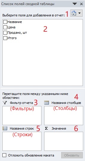
Let us pay special attention to one of the steps in compiling a summary table – the selection of fields and distribution by region. In order to understand the method of working with the “Table Fields” window, let’s consider its elements separately.

In newer versions of Microsoft Excel, the window looks slightly different, but the functionality is retained.

1. Formats of the “Table Fields” window. In the menu, you can choose which sections will be shown on the screen.
2. List of fields that are added to the report.
3. In the “Filters” field, you need to move the indicators to further filter the data.
4. The “Columns” field should contain instructions on what data to display in columns.
5. The purpose of the “Rows” area is almost the same as that of the “Columns” area – we specify the data that will be displayed in the rows.
6. In the “Values” area there should be fields with a number format for calculations.

If there is a lot of data in the sources, you can use the Defer Layout Update feature to prevent program errors.

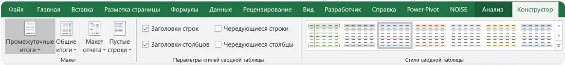
Table appearance customization

Changes to the appearance of a PivotTable are made using the tools on the Design tab. It appears on the control panel when the report has already been generated. The functions of the “Layout” section allow you to change the structure of the final table. The PivotTable Styles section contains different color themes that are applied to the report.

How to work with pivot tables in Excel

It may not be enough to create a report in the form of a table – additional steps are required. Consider several ways to work with a pivot table, its structure and data.

How to add a column or table to an Excel PivotTable

If you want to supplement the report with new information from the expanded range, you will have to change the cell selection.

1. Open the “Analysis” tab (in earlier versions – “Options”) and click on the “Data Source” button.

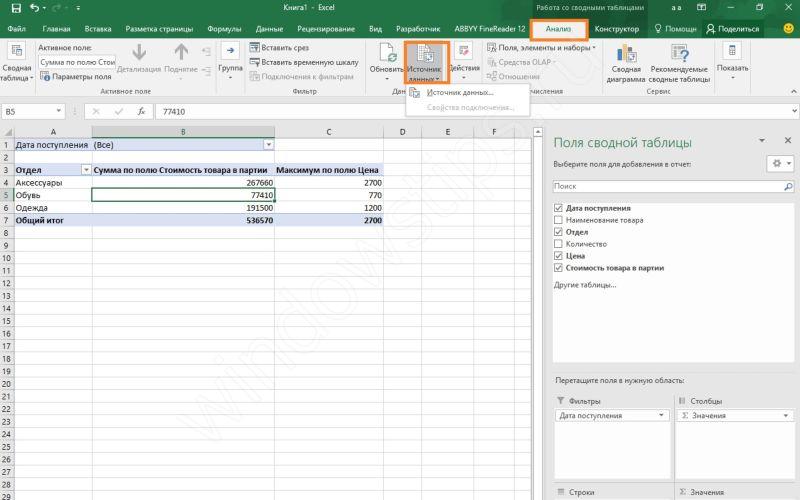
2. The initial table, according to which the report was compiled, and a window for selecting the range will appear on the screen. We add a column with new data to it and select a new range with the mouse.
3. Update the PivotTable – new fields will appear in the list. They need to be distributed by region.

Pay attention! It is not possible to make a new table a data source. If you want to add information from a table, you will need to create a new report on the same sheet and put two tables side by side.

Refresh data in a pivot table in Excel

If the report has not been converted to dynamic format, there are still ways to update the information in the report after changes have been made to the source. Let’s update the pivot table manually. To do this, click on any cell of the report and on the Refresh item in the context menu. You can also use the button with the same name on the “Parameters” / “Analysis” tab.

This tab contains a tool with which you can update the table automatically.

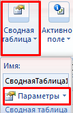
1. Select any cell of the report and open the “Parameters” / “Analysis” tab. We find the item “Pivot Table” – in it you need to select the item “Parameters”.

2. We find the item “Layout and format” in the settings. This section contains several items. It is required to check the boxes shown in the image below and click the “OK” button.

Conclusion

A report in a tabular format is quickly compiled thanks to Excel tools. Its visibility and breadth can be chosen at the drafting stage. The program allows you to change the structure and content of tables.