How to calculate percentage of a number in Excel. How to calculate share in excel

Actions with percentages are often performed in Microsoft Excel, it is quite convenient and practical. To do this, the program uses special formulas and functions. In this article, we will consider in detail all the ways to find out the percentage of a number.

Calculation of a share from a given number

Sometimes it is necessary to find out what is the proportion of one number in another. To do this, use the following formula: Share (%) = Number 1/Number 2*100%. The number 1 is the initial one, the Number 2 is the one in which the fraction of the number 1 is found. Let’s consider this mathematical operation with an example. Imagine that you need to find the fraction of the number 18 in the number 42. You need to perform a two-step algorithm:

1. Select an empty cell and write the formula there with the given numbers. An equal sign is required before the formula, otherwise the automatic calculation will not occur.

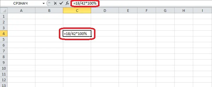
2. Press the “Enter” key, the cell will display the value of the calculation as a percentage or a regular number.

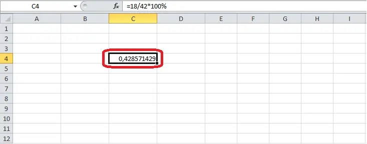
Important! It is not necessary to write the “*100” part in the formula. A fraction can be determined by simply dividing one number by another.

If the result is a number, not a percentage, you need to change the format of the cells. This can be done using the appropriate section in the Excel tools.

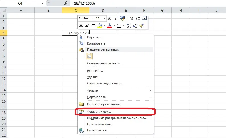
1. Click on the cell with the right mouse button. A menu will open where you need to select the “Format Cells” item.

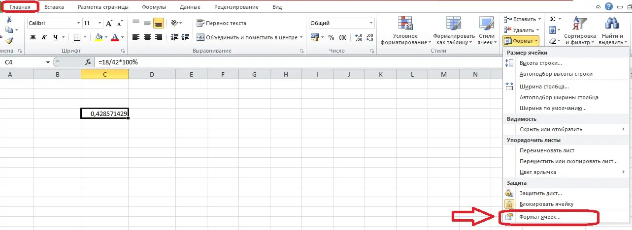
You can also find this option on the Home tab. There it is located in the “Cells” section (subsection “Format”).

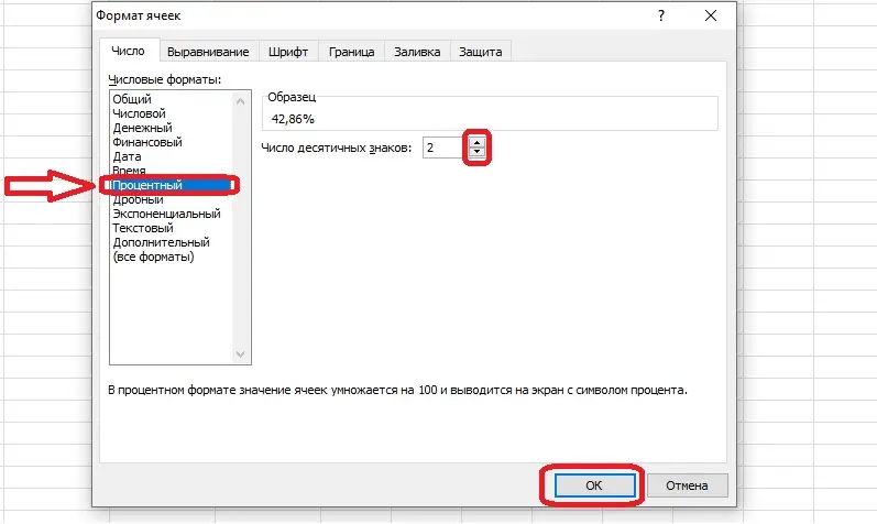
2. A menu with options to change the format will appear on the screen. In the “Number” tab there is a list of number formats – you need to select “Percentage”. By default, 2 decimal places are set, but this can be fixed with the arrow buttons. After completing the settings, click “OK”. Now the selected cell will always contain data in percentage format.

Let’s use the acquired knowledge on a more complex example. For example, you need to determine the share of each type of product in total revenue. To accomplish this task, we will compile a table where we indicate the unit price for several products, sales volumes and revenue. You also need to calculate the total revenue using the SUM function. At the end of the table, we will create a column for shares in total revenue with cells in percentage format. It is necessary to consider the calculation of this indicator step by step:

1. Select the first free cell in the last column and enter the share calculation formula in the field. The number 1 will be the income from the sales of one product, and the second – the sum of the total income.

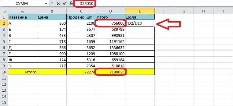
2. Press the “Enter” key, the percentage will appear in the cell.

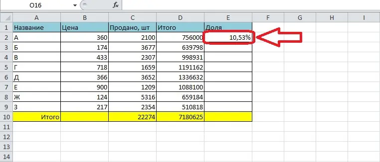
Next, you need to fill in the entire column with such data. It is not necessary to enter the formula manually every time – we automate the filling with a slight modification of the expression.

1. One component of the formula changes from line to line, the other remains the same. Let’s make sure that when the function is transferred to another cell, only one argument is replaced. You must click on the filled cell and insert dollar signs in front of the letter and number in the designation of the total revenue field through the formula bar. The expression should look something like this: =D2 / $D$ 10.
2. Next, select all the cells in the column up to the “Total” line by holding the lower right corner on the first cell. Each line contains information about the share of goods in total income.

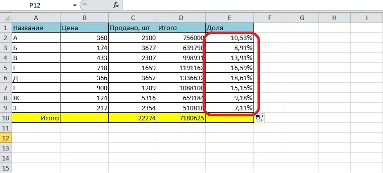
3. You can find out the share in the final revenue without calculating income. Let’s use the SUM function – the expression with it will replace the second argument.
4. Let’s create a new formula: =Revenue for one type of product/SUM(Revenue range for all products). As a result of the calculations, we get the same number as when using the previous method:

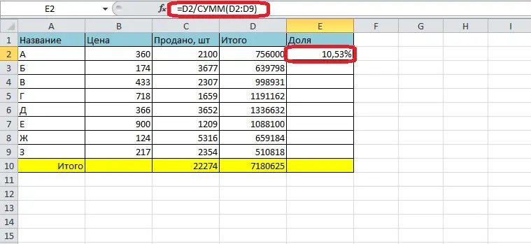
Calculating a percentage of a given number

The inverse operation – extracting a percentage of a number in a standard number format – is also often necessary. Let’s figure out how to carry out such a calculation. The calculation formula is: Number 2 = Percentage (%) * Number 1. The meaning of this expression: the percentage is determined from the Number 1, resulting in the Number 2. Let’s test the formula on a real example. It is necessary to find out how much it is – 23% of 739.

1. We select a free cell and compose a formula in it with known data.

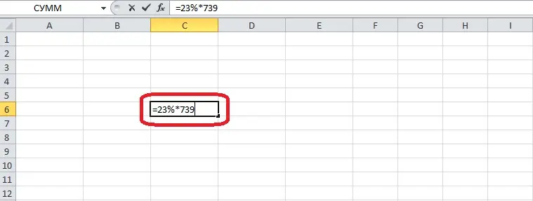
2. Press “Enter”, the result of the calculation appears on the sheet.

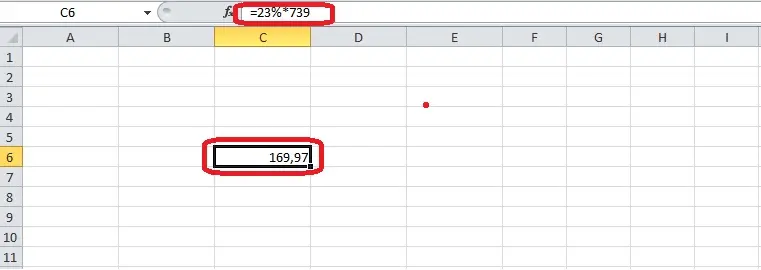
Pay attention! In this case, you don’t need to change the cell format because you want a number, not a percentage.

For the data example, you can use an already created table. Imagine that next month you plan to sell 15% more units of each product. It is necessary to find out what volume of production of different types of products corresponds to 15%.

1. We create a new column and enter the formula corresponding to the known data into the first free cell.

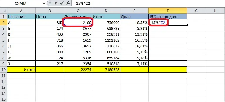
2. Press the “Enter” key and get the result.
3. We transfer the formula to all cells of the column using the fill handle.

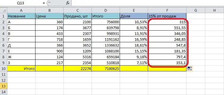
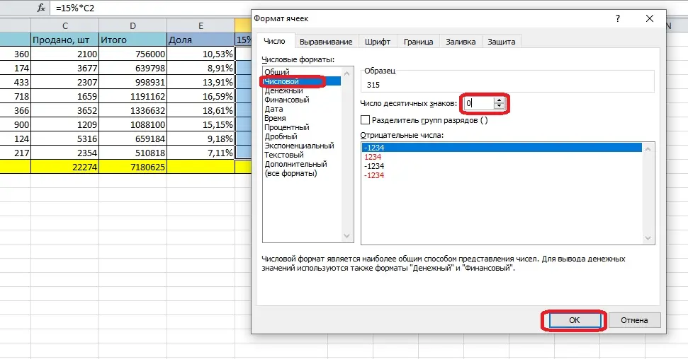
You can remove decimal places by changing the cell format. Select all cells with results, open the format menu and select Numeric. You need to reduce the number of decimal places to zero and click “OK”, after that the column will contain only integers.

Adding and subtracting interest

Based on the above formulas, you can perform simple mathematical operations with percentages.

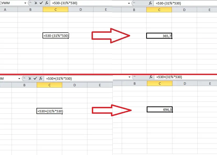
The calculation of the sum of the number and the percentage of it is as follows: Amount=Number+(Percentage (%)*Number). The difference formula differs only in sign: Difference=Number-(Percentage (%)*Number).

Consider these actions with examples – add 530% to 31, then subtract the same percentage from the initial number. You must select a free cell and enter the formula, then press “Enter”.

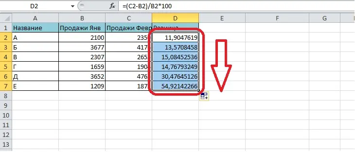
Excel tools allow you to calculate the difference between two numbers expressed as a percentage. The formula for this action is: Difference=(Number 2-Number 1)/Number 1*100%. 

We use the formula in the example: sales of goods have increased, and we need to determine by what percentage more units of products of different names were sold.

1. In a specially created column, select the top cell and write a formula in it. Numbers 1 and 2 are old and new sales.

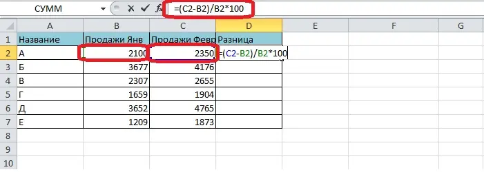
2. Press “Enter” and get the first result.
3. Select all cells of the column with the autocomplete marker – the formula is copied with an offset.

Conclusion

Working with percentages in Excel is quite easy, because the formulas are the same as the actions familiar to most from the mathematics course. However, it is much more convenient to calculate interest in the program, because it is possible to automate the calculations.