Subtotal function in Excel. Formula, table requirements

Intermediate results that need to be obtained when compiling reports can be easily calculated in Excel. There is a fairly convenient option for this, which we will consider in detail in this article.

Requirements that apply to tables in order to obtain intermediate results

Subtotal function in Excel is only suitable for certain types of tables. Later in this section, you will learn what conditions must be met in order to use this option.

1. The plate should not contain empty cells, each of them must contain some information.
2. The header should be one line. In addition, its location must be correct: without jumps and overlapping cells.
3. The design of the header must be done strictly in the top line, otherwise the function will not work.
4. The table itself should be represented by the usual number of cells, without additional branches. It turns out that the design of the table must consist strictly of a rectangle.

If you deviate from at least one stated requirement when trying to use the “Intermediate results” function, errors will appear in the cell that was selected for the calculations.

How the subtotal function is used

To find the necessary values, you need to use the corresponding function, which is located at the top of the Microsoft Excel sheet on the top panel.

1. We open the table that meets the requirements specified above. Next, click on the table cell, from which we will find the intermediate result. Then go to the “Data” tab, in the “Structure” section, click on “Subtotal”.

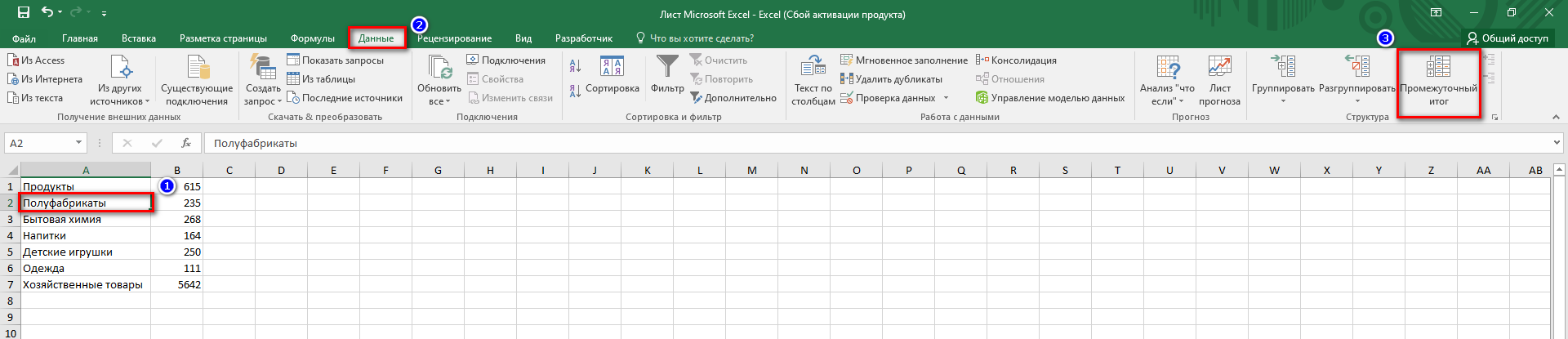
2. In the window that opens, we need to select one parameter, which will give an intermediate result. To do this, in the “At each change” field, you must specify the price per unit of goods. Accordingly, the value is put down “Price”. Then press the “OK” button. Please note that in the “Operation” field, you must set the “Amount” in order to correctly calculate the intermediate values.

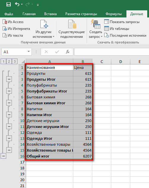
3. After clicking on the “OK” button in the table for each value, a subtotal will be displayed, shown in the screenshot below.

On a note! If you have already received the required totals more than once, then you must check the box “Replace current totals”. In this case, the data will not be repeated.

If you try to collapse all the lines with the tool set to the left of the plate, you will see that all intermediate results remain. It was them that you found using the instructions above.

Subtotals as a formula

In order not to look for the necessary function tool in the tabs of the control panel, you must use the “Insert function” option. Let’s consider this method in more detail.

1. Opens a table in which you need to find intermediate values. Select the cell where intermediate values ​​will be displayed.

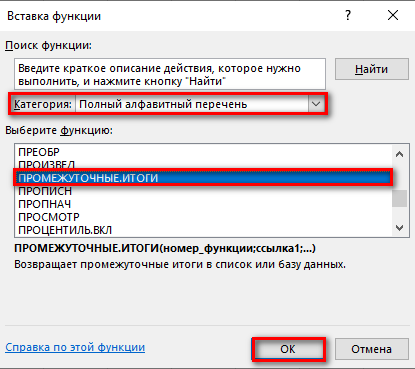
2. Then click on the “Insert Function” button. In the window that opens, select the required tool. To do this, in the “Category” field, we are looking for the “Full alphabetical list” section. Then, in the “Select a function” window, click on “SUB.TOTALS”, click on the “OK” button.

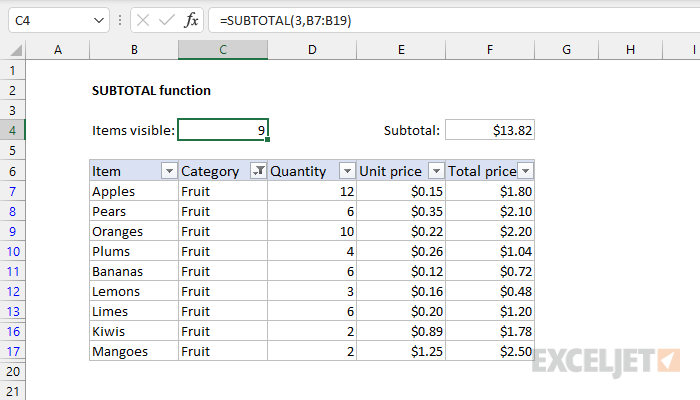
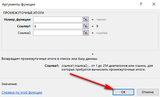
3. In the next window “Function arguments” select “Function number”. We write down the number 9, which corresponds to the information processing option we need – the calculation of the amount.

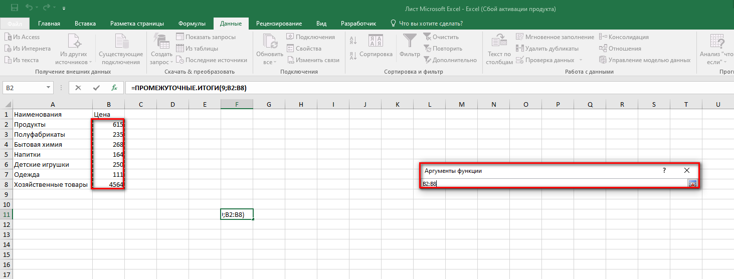
4. In the next data field “Reference”, select the number of cells in which you want to find subtotals. In order not to enter data manually, you can simply select the range of required cells with the cursor, and then click the OK button in the window.

As a result, in the selected cell, we get an intermediate result, which is equal to the sum of the cells we selected with the written numerical data. You can use the function without using the “Function Wizard”, for this you must manually enter the formula: =SUBTOTALS(number of data processing, cell coordinates).

Pay attention! When trying to find intermediate values, each user must choose their own option, which will be displayed as a result. It can be not only the sum, but also the average, minimum, maximum values.

Applying a Function and Processing Cells Manually

This method involves applying the function in a slightly different way. Its usage is presented in the algorithm below:

1. Launch Excel and make sure the table is displayed correctly on the sheet. Then select the cell in which you want to get the intermediate value of a specific value in the table. Then click on the button under the control panel “Insert function”.

2. In the window that appears, select the category “10 recently used functions” and look for “Intermediate totals” among them. If there is no such function, accordingly it is necessary to prescribe another category – “Full alphabetical list”.

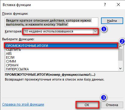
3. After the appearance of an additional pop-up window where you need to write “Function Arguments”, we enter there all the data that was used in the previous method. In such a case, the result of the “Subtotals” operation will be performed in the same way.

In some cases, to hide all data, except for intermediate values ​​in relation to one type of value in a cell, it is allowed to use the data hiding tool. However, you need to be sure that the formula code is written correctly.

To summarize

Subtotal calculations using Excel spreadsheet algorithms can only be performed using a specific function, but it can be accessed in a variety of ways. The main conditions are to perform all the steps in order to avoid mistakes, and to check whether the selected table meets the necessary requirements.