


Contents
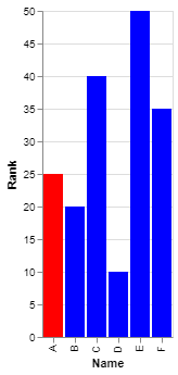
Suppose we have built a simple histogram to visually display values for several categories – for example, profit by branch cities:

Task: highlight the desired column(s) according to the specified condition, for example, the city with the highest sales or the city selected in the drop-down list, etc. And to do this not by manually changing the color of the column fill, but “on autopilot”, because. Tomorrow the data will change and the backlight should also be updated. In other words, you need to implement something like conditional formatting, but not for cells, but for columns in the chart.
The essence of the method
The idea is actually simple. Let’s add one more auxiliary column to our data table:

Note that:
- Opposite the city that we want to highlight (in the example – Korolev) is worth its own value.
- In all other lines, we intentionally create the #N/A! using the function ND() no arguments (in the English version – NA ())
If we now build a histogram according to such a table or add an auxiliary column as a new series to the existing chart, then we will see the same picture, but the column we need will be duplicated in the new data series:

Now the main thing: right-click on any column, select the command Data series format (Format Data Series) and in the window that appears, move the slider overlapping rows (Overlap) at 100%:
 |  |
The duplicate column will run over the original one, completely overlapping it, but, in fact, it will look like highlighting the specified column. And the cells in which there are any errors on the charts are not displayed. Instead of ND, you can also display an empty string “” – the effect is about the same.
Well, if you use formulas in an additional column, then you can implement highlighting according to any criteria – there is a lot of room for imagination here. Let’s take a look at some seeding examples.
Highlighting a column in a chart with a selection from a dropdown list
Suppose we made a drop down list in cell G2 to select the desired city using the classic command Data – Data Validation (Data — Data Validation) and sourced our list of cities A2:A15:

Now you can enter a simple formula in the auxiliary highlight column that will highlight the selected city:

It is easy to imagine that the function IF (IF) checks if this is the city we need and displays its value or generates a #N/A error.
Highlight the largest or smallest column
Very similar to the previous method, but with the function IF check in turn whether the value of sales for each city is equal to the maximum in the column:

Of course, you can function MAX replaced by ME.
Highlight columns above/below average
And if we replace the equal sign with more or less in the previous formula, and the function MAX on AVERAGE (AVERAGE), then you can highlight all cities where sales were above or below the national average:

Backlight Top-3
If instead of the MAX function, which finds only one largest value, use the function LARGE (LARGE), you can easily highlight Top-3:

Well, and so on – I think you already got the idea.
- How to build a chart in Excel, where the width of the columns is a variable and also makes sense
- Several Ways to Visualize Plan-Act Ratio on a Chart in Excel
- How to quickly add new data series to a finished chart