ATAN (arctangent) function in Excel

Arctangent is a trigonometric function inverse to tangent, which is used in the exact sciences. As we know, in Excel we can not only work with spreadsheets, but also make calculations – from the simplest to the most complex. Let’s see how the program can calculate the arc tangent from a given value.

We calculate the arc tangent

Excel has a special function (operator) called “ATAN”, which allows you to read the arc tangent in radians. Its general syntax looks like this:

=ATAN(number)

As we can see, the function has only one argument. You can use it in different ways.

Method 1: Entering the formula manually

Many users who often perform mathematical calculations, including trigonometric ones, eventually memorize the function formula and enter it manually. Here’s how it’s done:

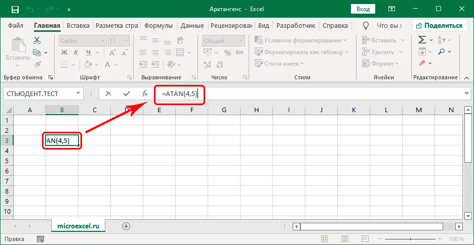
1. We get up in the cell in which we want to make a calculation. Then we enter the formula from the keyboard, instead of the argument we specify a specific value. Do not forget to put an “equal” sign before the expression. For example, in our case, let it be “ATAN(4,5)”.
2. When the formula is ready, click Enterto get the result.

Notes

1. Instead of a number, we can specify a link to another cell containing a numeric value. Moreover, the address can be entered either manually, or simply click on the desired cell in the table itself.

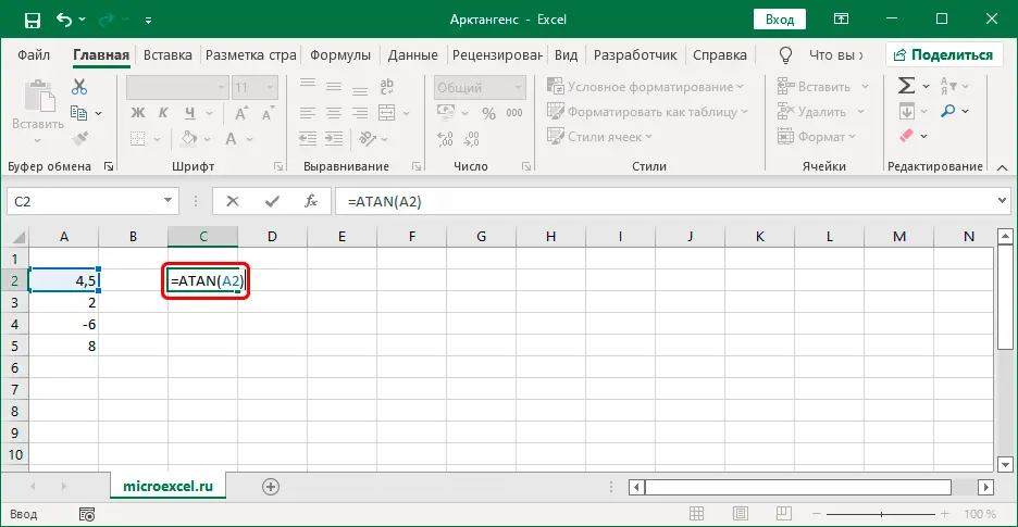
This option is more convenient because it can be applied to a column of numbers. For example, enter the formula for the first value in the corresponding line, then press Enterto get the result. After that, move the cursor to the lower right corner of the cell with the result, and after a black cross appears, hold down the left mouse button and drag down to the lowest filled cell.

By releasing the mouse button, we get an automatic calculation of the arc tangent for all initial data.

2. Also, instead of entering the function in the cell itself, you can do it directly in the formula bar – just click inside it to start the editing mode, after which we enter the required expression. When ready, as usual, press Enter.

Method 2: Use the Function Wizard

This method is good because you do not need to remember anything. The main thing is to be able to use a special assistant built into the program.

1. We get up in the cell in which you want to get the result. Then click on the icon “Fx” (Insert Function) to the left of the formula bar.
2. A window will appear on the screen. Function Wizards. Here we select a category “Full alphabetical list” (or “Mathematical”), scrolling through the list of operators, mark “ATAN”, then press OK.
3. A window will appear for filling in the function argument. Here we specify a numeric value and press OK.As in the case of manually entering a formula, instead of a specific number, we can specify a link to a cell (we enter it manually or click on it in the table itself).
4. We get the result in a cell with a function.

Note:

To convert the result obtained in radians to degrees, you can use the function “DEGREES”. Its use is similar to how it is used “ATAN”.

Conclusion

Thus, you can find the arc tangent of a number in Excel using the special ATAN function, the formula of which can be immediately entered manually in the desired cell. An alternative way is to use a special Function Wizard, in which case we do not have to remember the formula.