Contents
The main work of the office program Excel focuses on formulas. With their help, you can process a wide variety of data with different levels of complexity, as well as perform mathematical operations, both simple arithmetic and very complex, from the category of higher mathematics.
However, a novice user does not always know how to correctly perform such a simple task as summing cells. There is nothing surprising in this, since all of us at one time or another in our life did not know how to do this or that. Therefore, today let’s figure out how to calculate the sum of a column in Excel. And we have four ways to do it.
Calculating sums in columns in various ways
There are several methods for determining the sum of values in Excel columns. There are both automatic and manual, using the built-in functionality of the application. In addition, it is not necessary to write the final result in a cell to see it, there is a way to immediately determine what the sum of all values in the cell will be. Let’s start with a simpler method, and then gradually move on to more complex ones.
Viewing the entire amount
If we just want to find out the sum of all the numbers in a column where the cells contain specific values and there is no need to save it for later use in formulas, we should follow these steps:
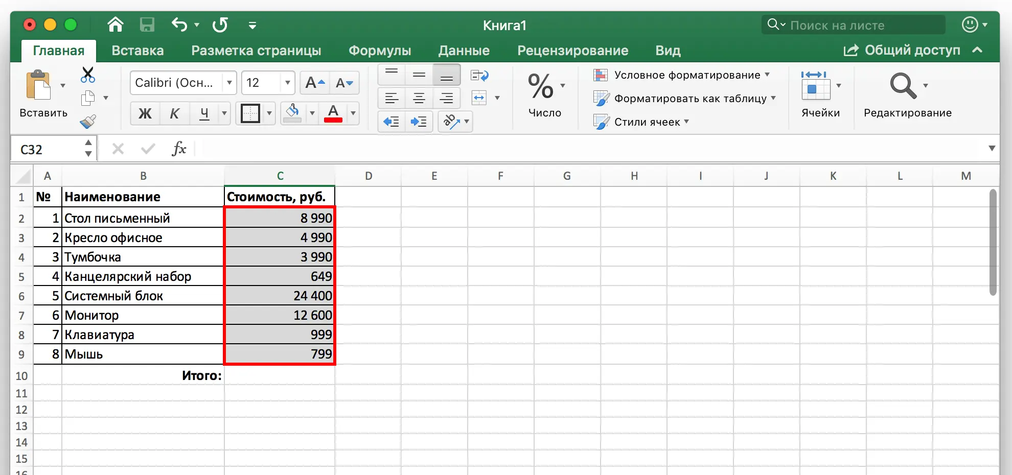
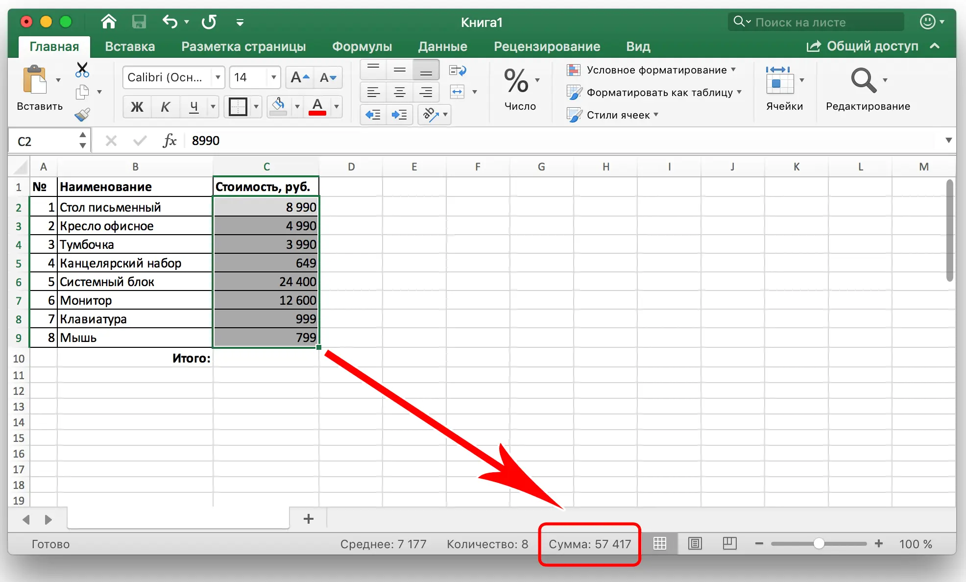
- Left-click on the first cell of the range in which you want to perform an arithmetic operation, and then select by dragging all the necessary cells. You can also select them one by one, skipping some by holding down the Ctrl key and successively clicking on each of the cells that you want to select. After selection, we get the following result.

- Now we need to look at the status bar, where the result will be contained. Moreover, even if a row of cells in a column does not contain any values, this method will still work.

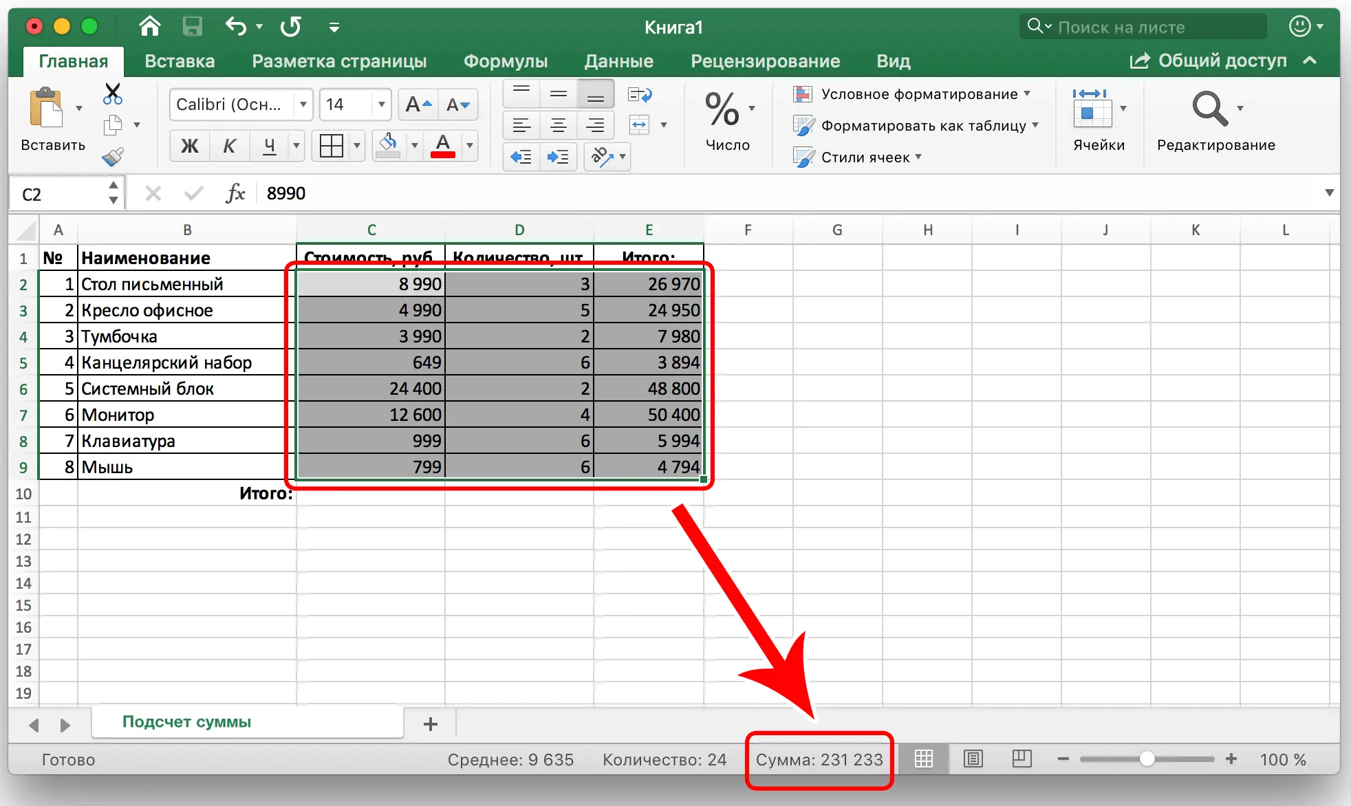
- In the same way, you can count in several columns at once. To do this, you need to select the appropriate range of values, and then look at the resulting value below.

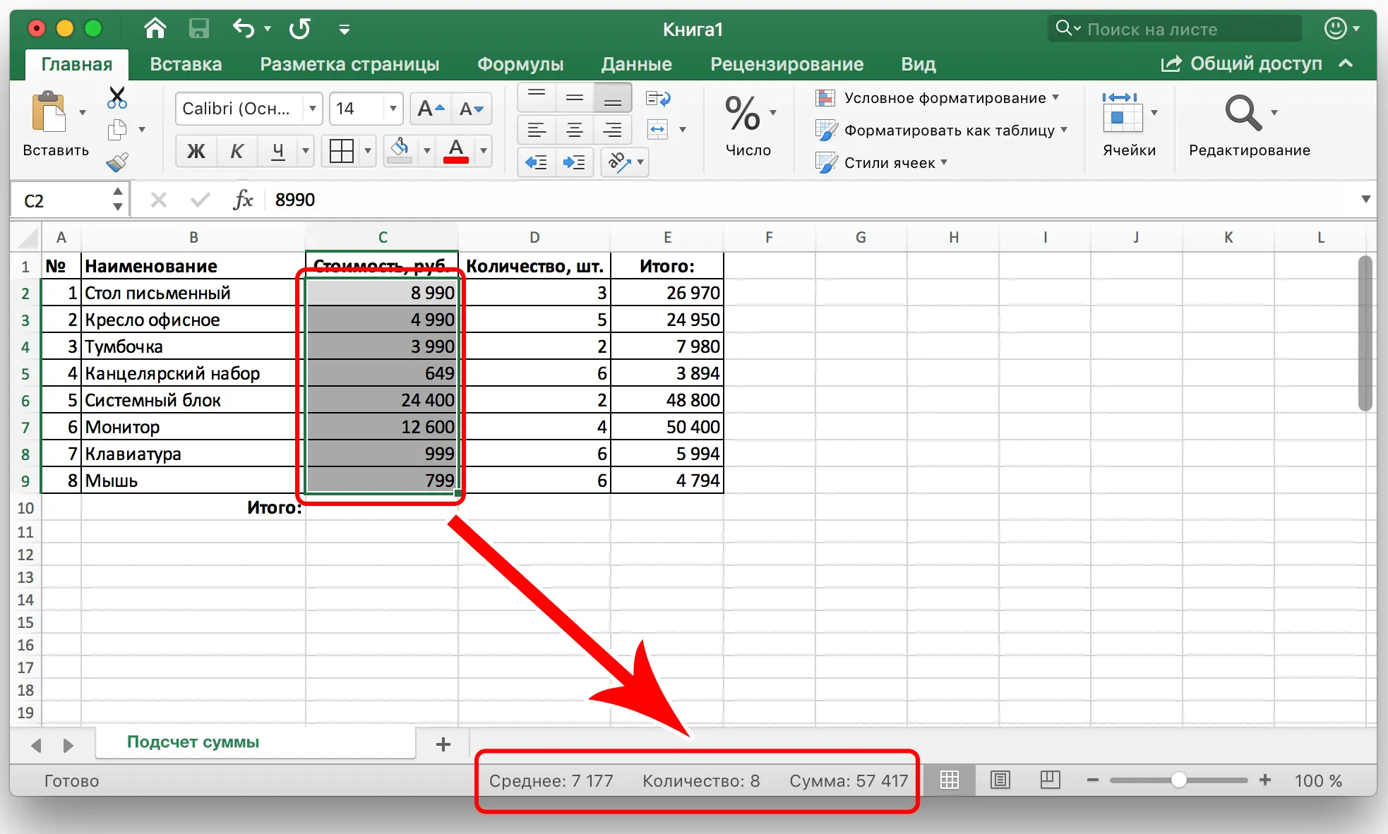
- You can also find out the average value of all selected cells, their total number is slightly to the left.

Autosummation
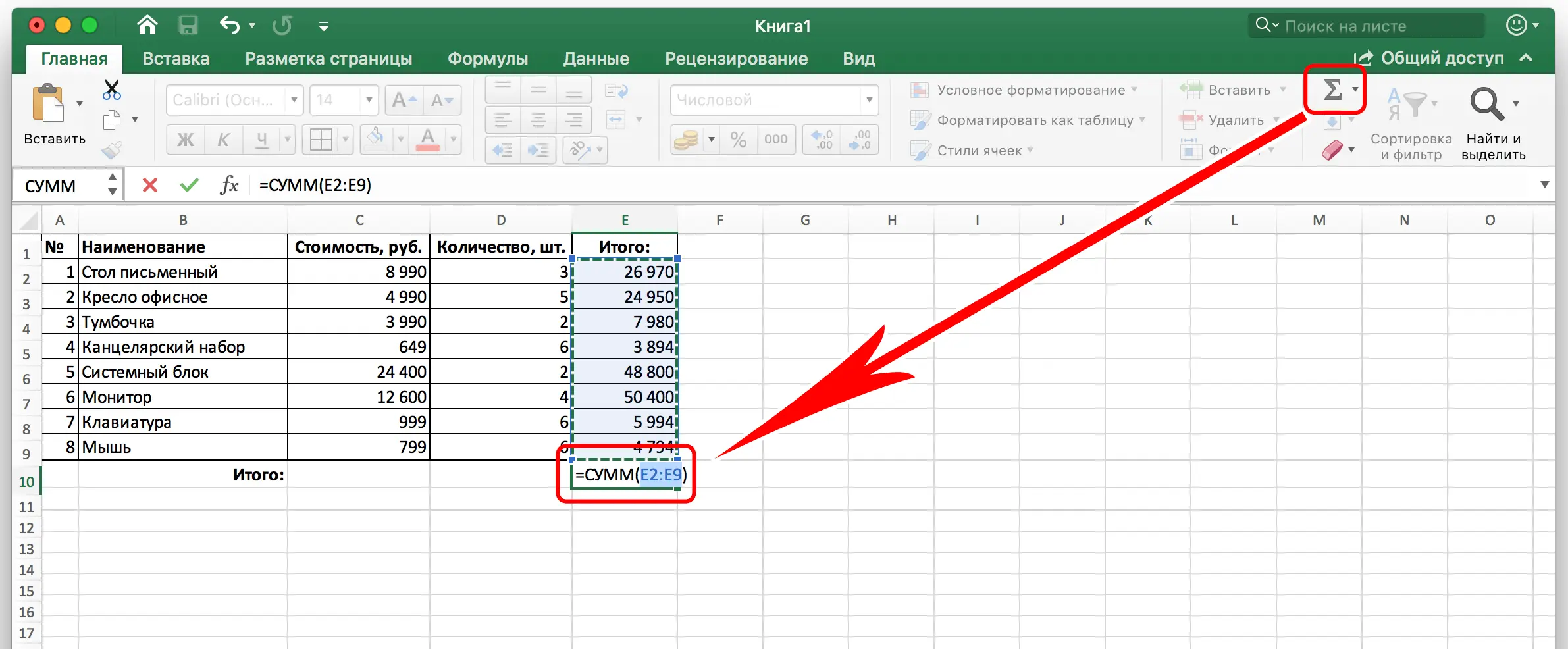
Often you need to fix the sum of numbers for columns in a separate cell. This is necessary so that it can be used in other calculations. In such situations, the optimal solution is automatic summation. To implement it, you must perform the following steps:
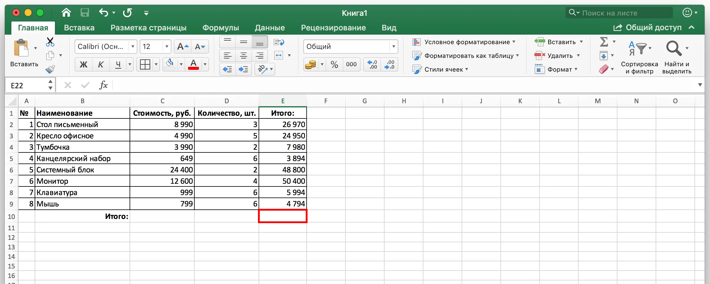
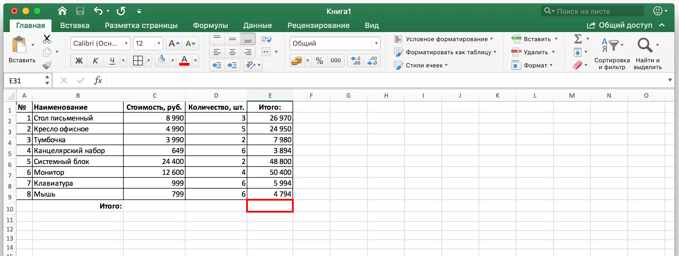
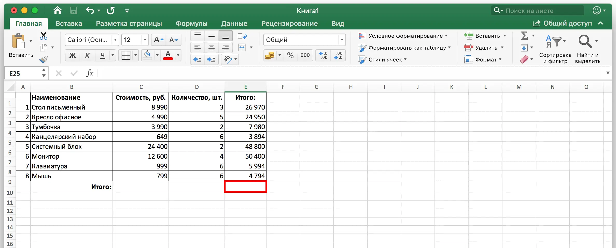
- Left-click on an empty cell. It can be located anywhere, but it is optimal to select a separate line with a separate cell. It looks aesthetically pleasing and functional.

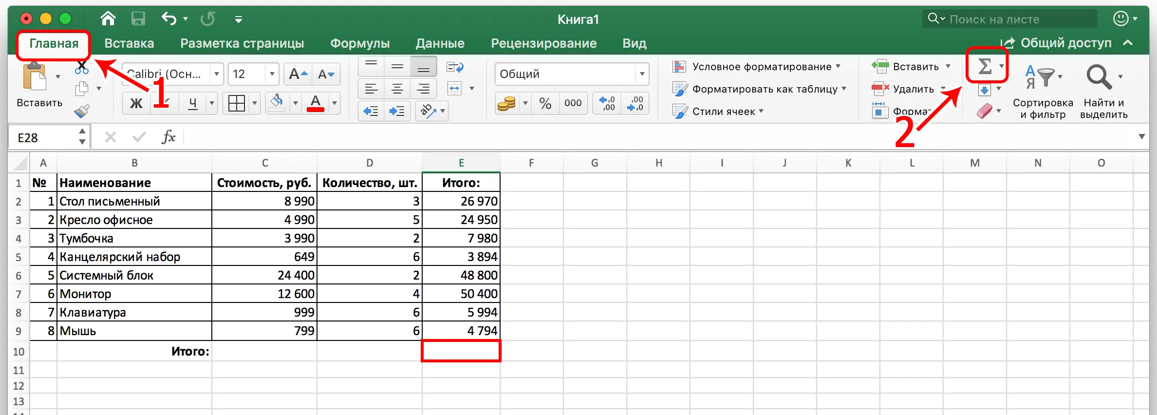
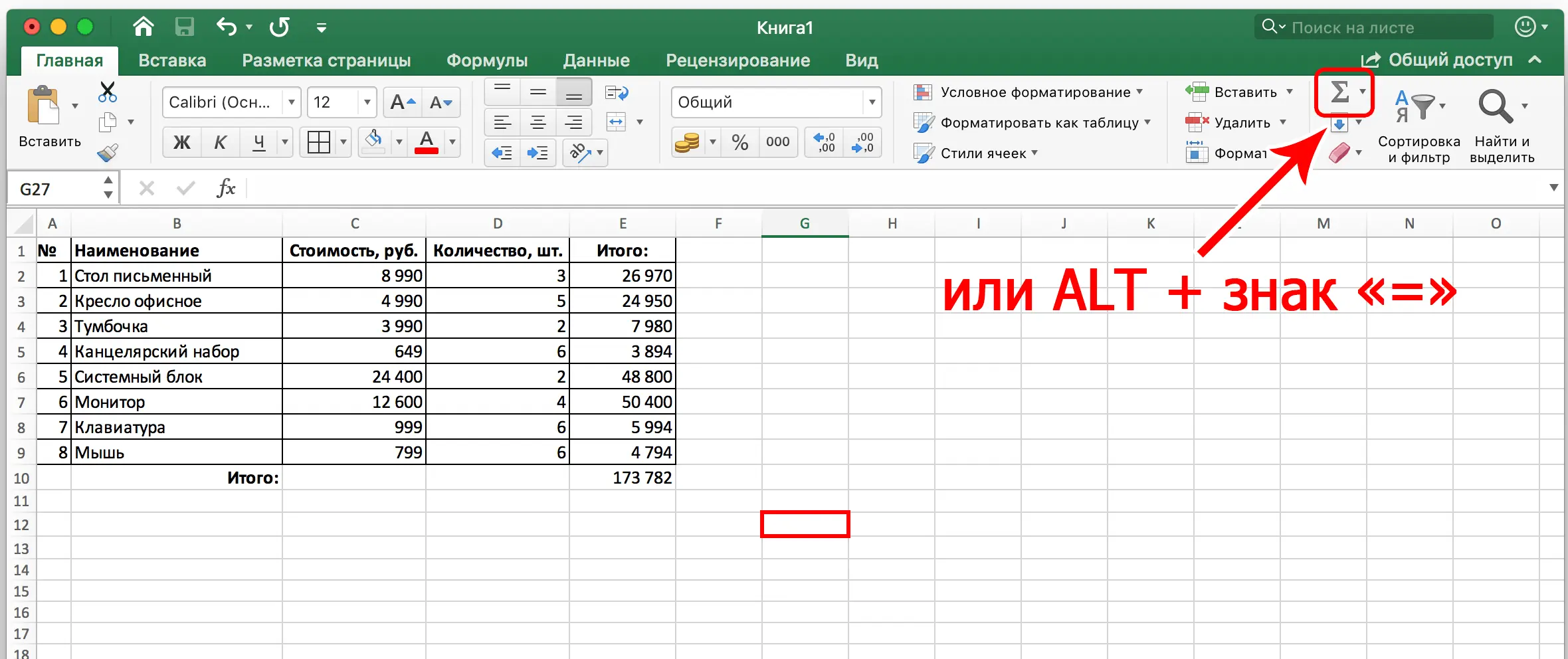
- Next, make a left mouse click on the “Amount” button. It can be found on the right side of the ribbon if you open the Home tab. In addition, you can use a combination of hot keys. If you press the Alt button + the = sign at the same time, you can also get a similar result.

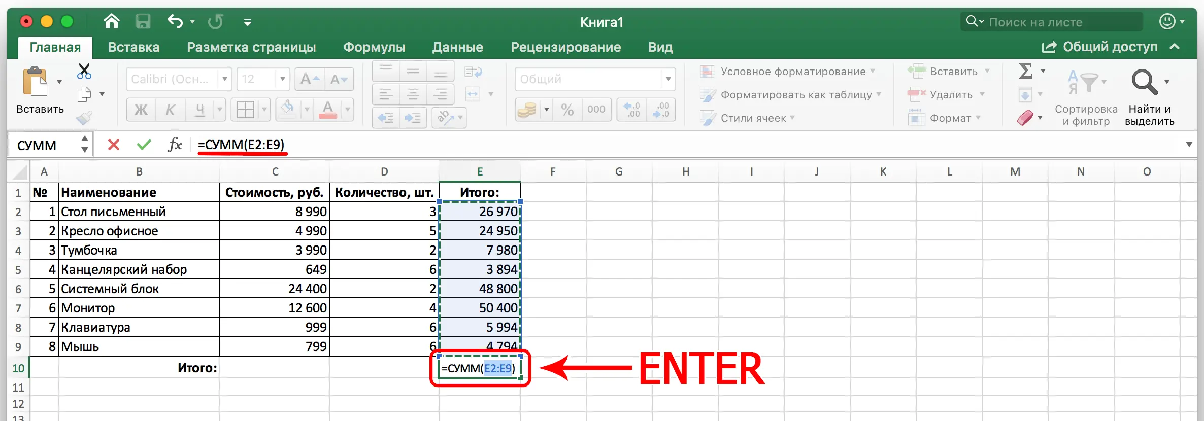
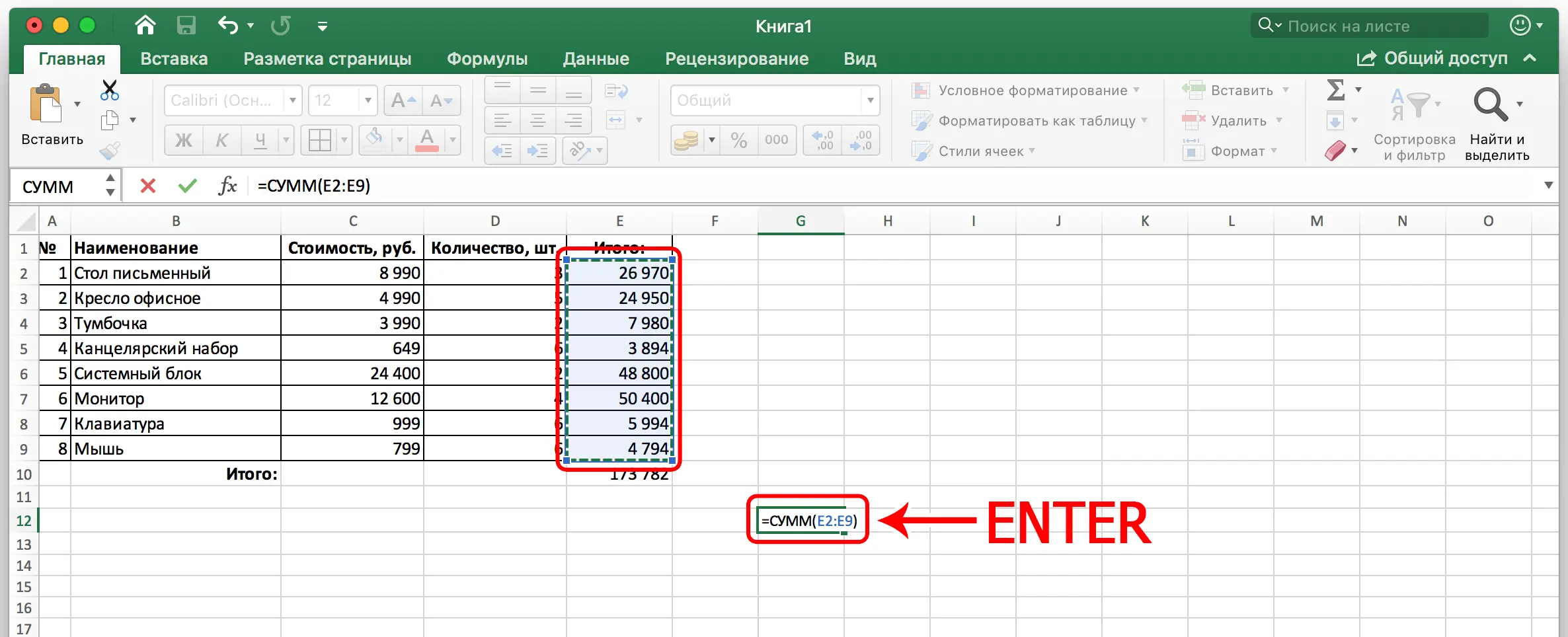
- Next, we need to make sure that this cell specifies the first and last cells of the summation range. If so, then confirm the action by pressing the Enter key.

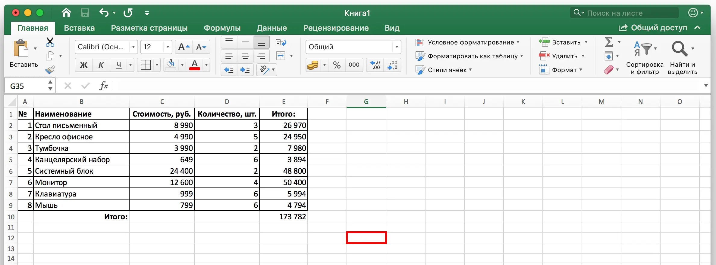
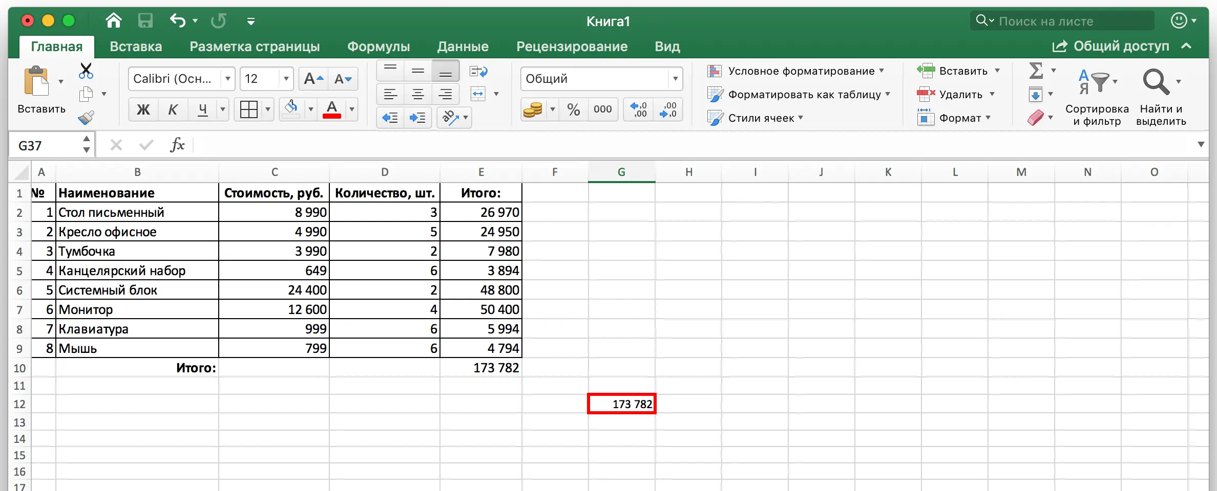
- Next, the sum of the numbers in the cell that we designated earlier will appear. Attention! If you make any changes to the original range, the amount will automatically change. That is, you do not need to manually repeat the input of the formula. All cells will be updated automatically.
Sometimes you need to make a count in another cell. In this case, the actions are similar, except that you need to select any other cell. It is possible to use for calculations even the cell that is in another column and even on another sheet. In general, the sequence of actions is as follows:
- Select the cell where you want to calculate the amount.

- Next, we find the same “Amount” button as in the example above. Well, or use the hot keys written in the screenshot.

- Next, using the left mouse button, select those cells whose summation is required and press the “Enter” key.

- Another selection method that can be used is to left-click on the cell that you want to select, and then click with the Shift key pressed on the last cell of this range.
- As a result, we get such a picture.

To sum the values of several columns with this method, you need to perform approximately the same sequence of actions. Again, the method will work anyway, even if there are some empty cells in the range that the user has selected.
Autosummation
Sometimes you need to take into account several columns at once in automatic mode. The mechanics of actions are very similar, but there is one difference, because of which this method needs to be separated into a separate subsection.
- We make a left mouse click on the cell in which we need to get the amount.

- Next, we shift our gaze to the toolbar, where we find the “Amount” button. Or use the keyboard shortcut above.

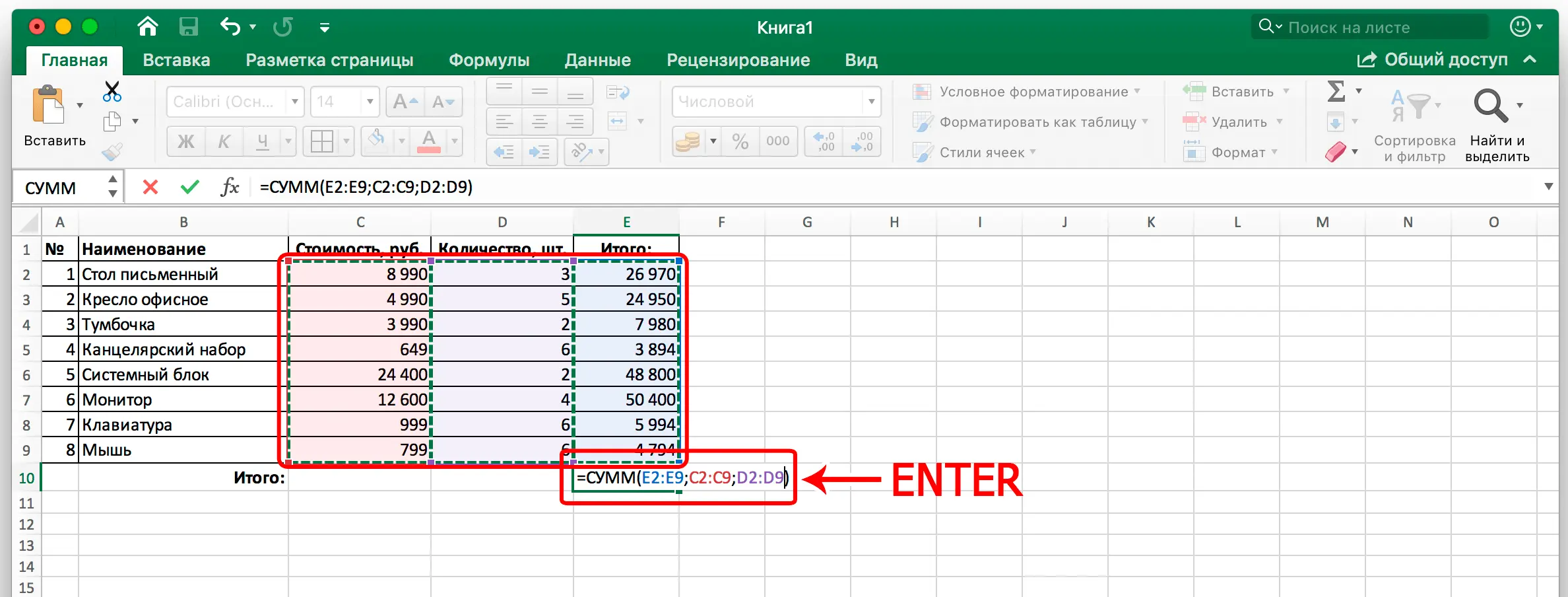
- The selection of the first column above the formula will be carried out automatically. Therefore, we need to select the remaining range in another column. To do this, use the Ctrl key, which we hold down during this entire time.

- If you need to determine the sum of cell values that are part of several columns that are next to each other, you can select all together in the same way as cells in one column. It’s just that the mouse cursor needs to be moved from the upper left corner of the range to the lower right, diagonally. Otherwise, there is no difference.

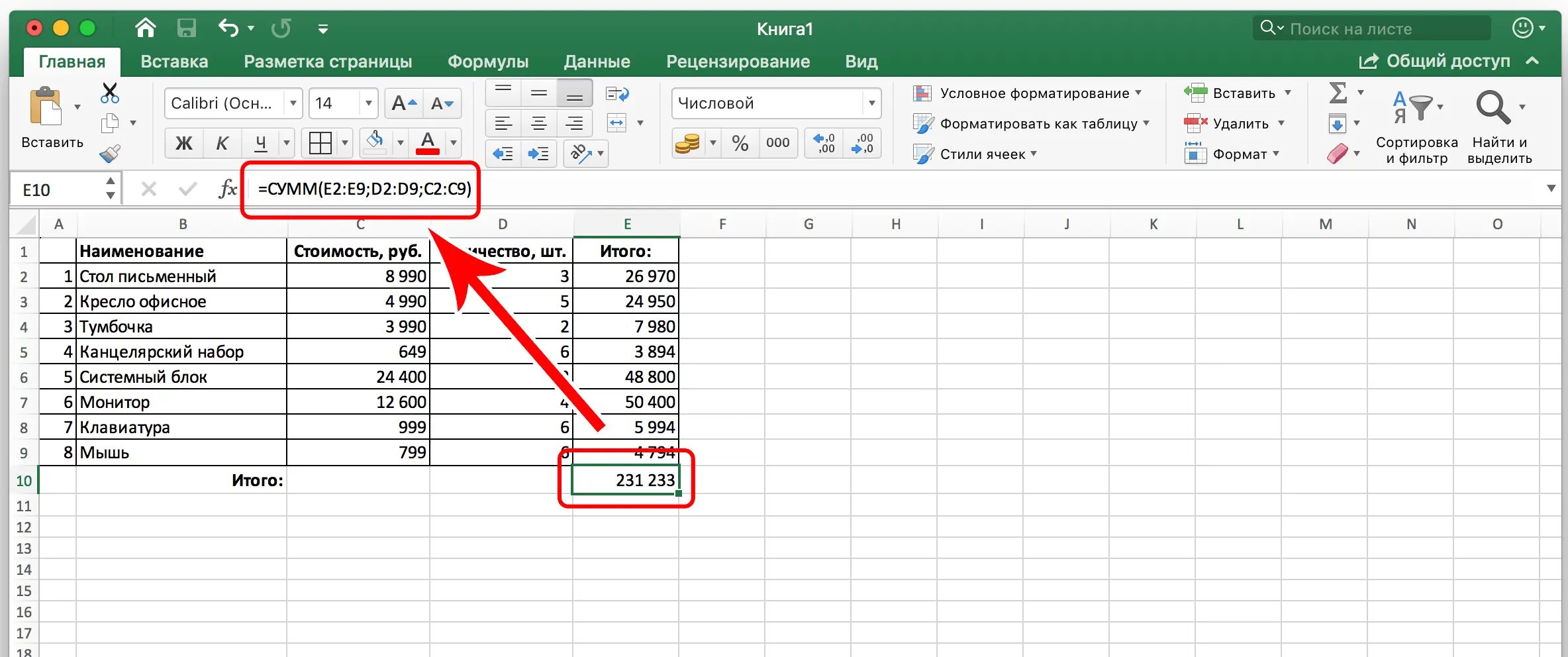
- After that, press the “Enter” key, and we will immediately see the result. The formula itself, which was used for calculations, we can see in the formula input line. And in the cell – the result.

Exactly the same actions must be carried out in order to determine the sum of the numbers contained in specific cells belonging to different columns. To do this, you need to click on the left mouse button, select the cell in which the sum of values uXNUMXbuXNUMXbshould be displayed, then click on the corresponding button on the toolbar (or use hot keys) and select the first set of cells. After that, holding down the Ctrl key, select the second range. Then we press “Enter”, after which the correct result is displayed in the appropriate cell.
If you double-click on it, we will immediately see the formula that was used for the calculations. It can also be entered manually. If a person owns a blind printing method, then this option may be much more convenient for him.
Manual finding of the sum
In general, this method is somewhat more inconvenient for the average person who does not have much experience with Excel. But in general, any more or less experienced computer user who uses the keyboard will say that often the keyboard is a much more effective tool for controlling the program than the mouse. Especially if the trackpad is used as a cursor control.
What do we need to do in order to carry out the summation manually. The first way is to sum each cell in turn. That is, enter the formula sign =, then click on the cell, then write +, then click on the second cell with the mouse. This method is not bad in situations where the number of cells is small. But it does not perform very well when there is too much data to process.
What is the other advantage of manually finding the sum? For example, when selecting individual cells or an entire range, errors can often occur. And fixing it is already much more difficult. Or rather, not more difficult, but less effective, since you still need to switch to the formula editing mode and edit everything manually. If the mistake was made at the manual stage of entering the formula, then it can be very easily corrected, just like any mistake when typing. There is no need to do everything from scratch, you just need to slightly adjust the entered data.
In addition, independent writing of the formula makes it easier to display the sum in different places in the table. Moreover, this method is useful if you need to place it on another sheet. This method makes it possible to sum up all possible combinations of cells, both whole ranges and individual cells located on different sheets. In this case, it is possible to exclude from accounting those cells that we will not take into account in the calculation.
To automate the manual calculation of large data sets (no matter how strange it may sound at first glance), you need to use the function SUM. We’ve seen it before, because the summation tool described above actually helps us populate this function with the right arguments. But you can also enter it manually.
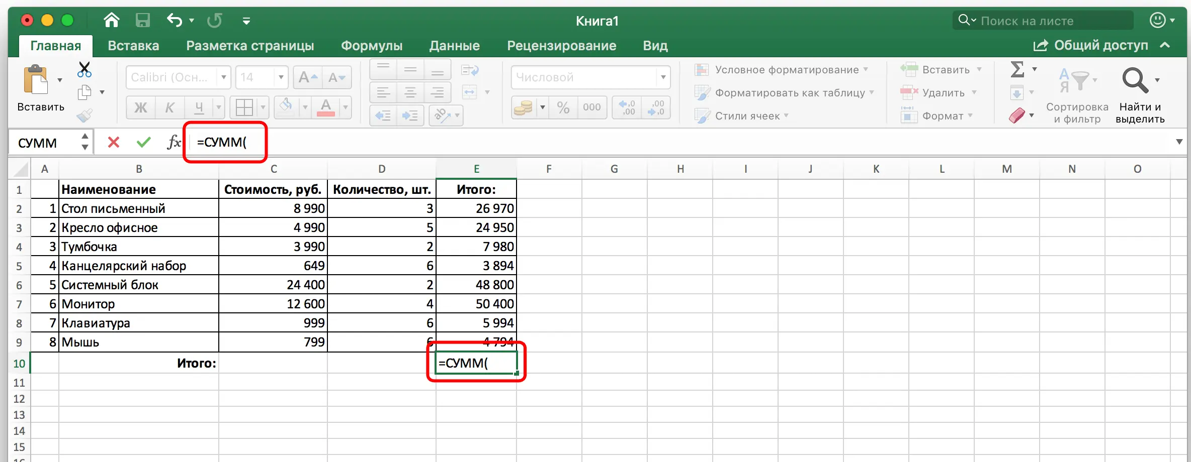
Its generic syntax is as follows: = SUM (added cells or range of cells). That is, all the data to which we need to apply the addition operation must be written in brackets. The value should look like this.
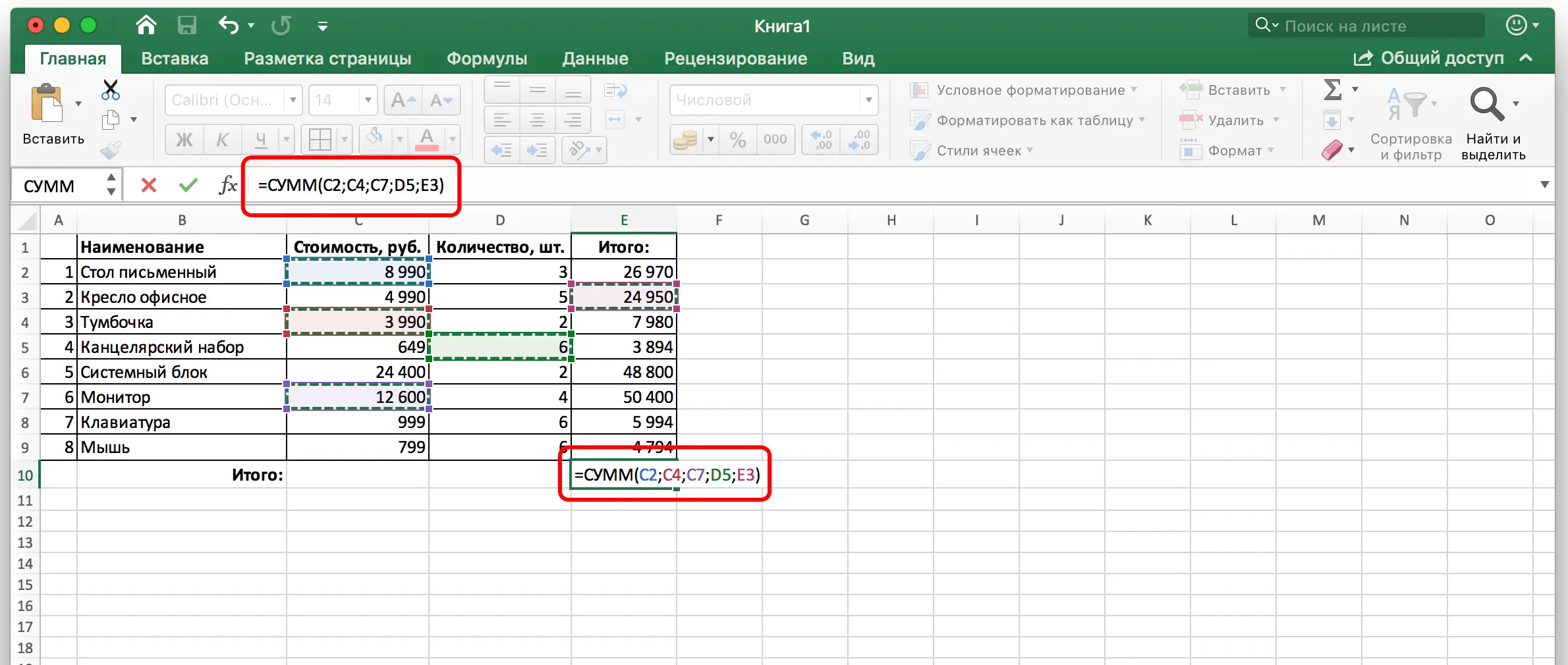
If we know which specific cells we need to add, and they are separate from each other, then they need to be listed separated by a semicolon. For example, if we use such cells as arguments, then the summation is applied to the values of column A, which have a numerical index of 2, 5, 7, 10. The addresses in this case will be as follows: A2; A5; A7; A10.
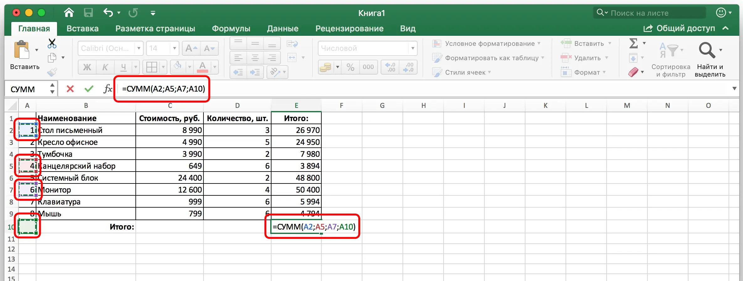
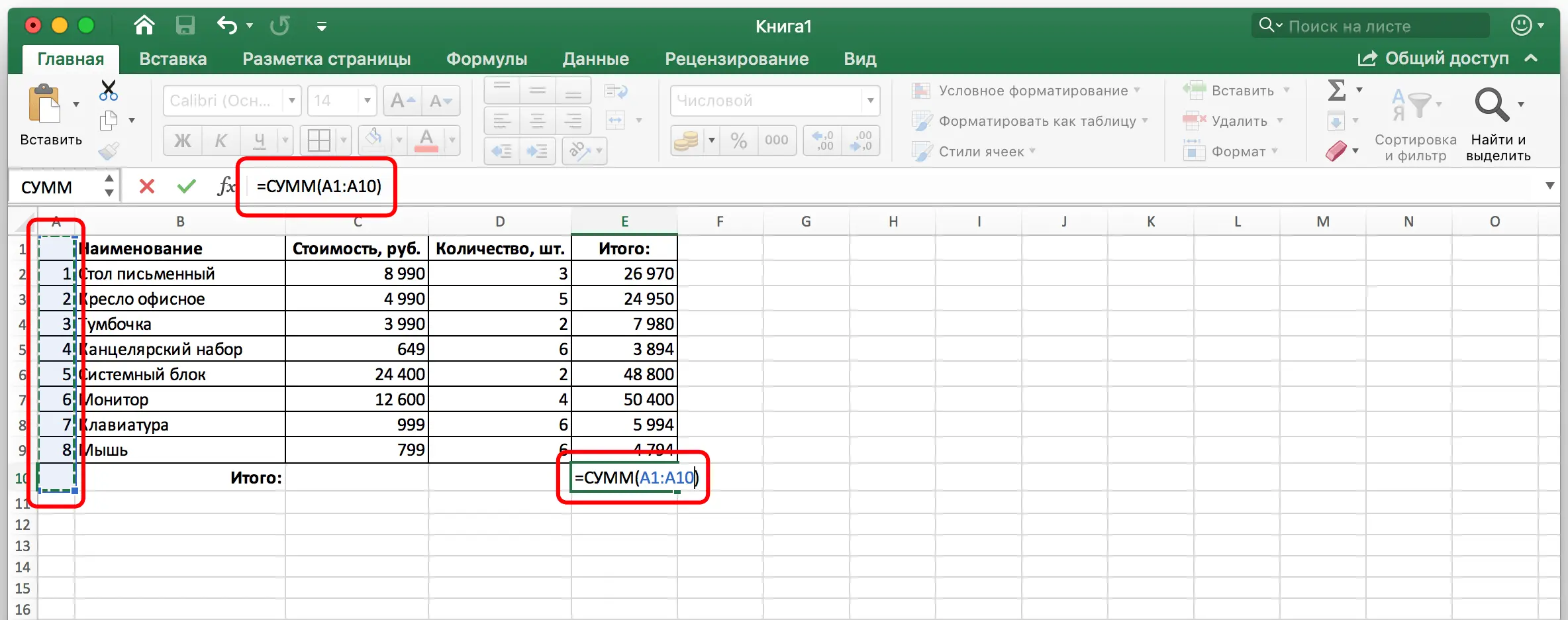
If we need to apply the summation to a range, then in this case we must first write the first cell, then put a colon, and then the last cell. For example, A1:A10. An example of such a recording method can be seen in this screenshot.
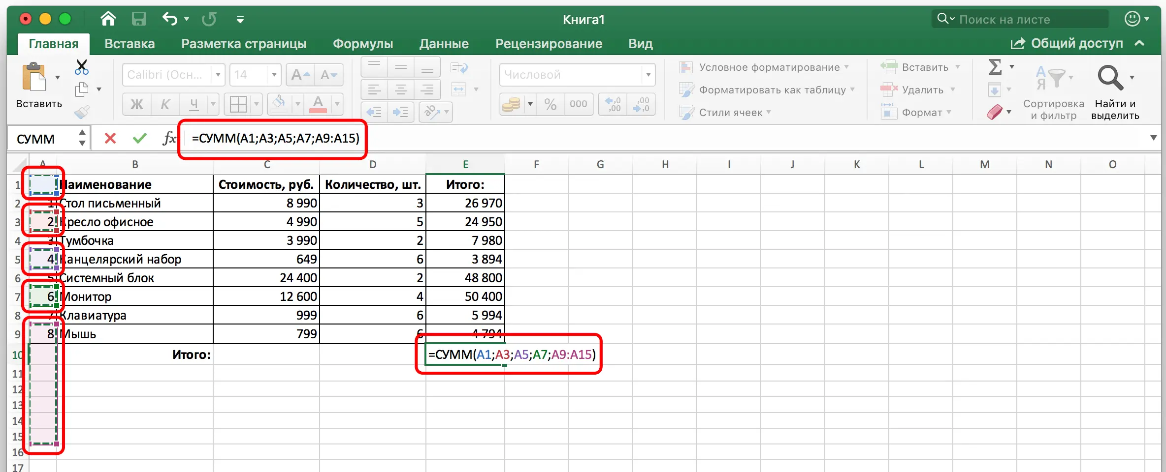
Also, the calculation can be mixed. In this case, both specific cells and ranges are used as arguments. In this case, cells and ranges are separated by semicolons. For example, like this. A1; A3; A5; A7; A9:A15. In this example, we see that the cells belonging to column A with numbers 1,3,5,7 are summed up, as well as a range of cells with numbers from 9 to 15. It is important to note that there should not be extra separators between specific cells and the range. There is only one separator – a semicolon. There are no special ones.
So, we need to perform the following steps to add values manually:
- Select a cell using the left mouse button. The cell in which the final value will be displayed should be highlighted.

- After that, we put the formula input sign (in Excel, this is the = sign, which is at the beginning of the formula input line), after which we write the name of the function and write the argument input sign (open bracket).

- After that, we write the arguments in accordance with the rules described above. Be sure to use separators. Semicolons are used to separate cells and ranges. A range is denoted by a colon (:), which separates the start and end of the selected range).

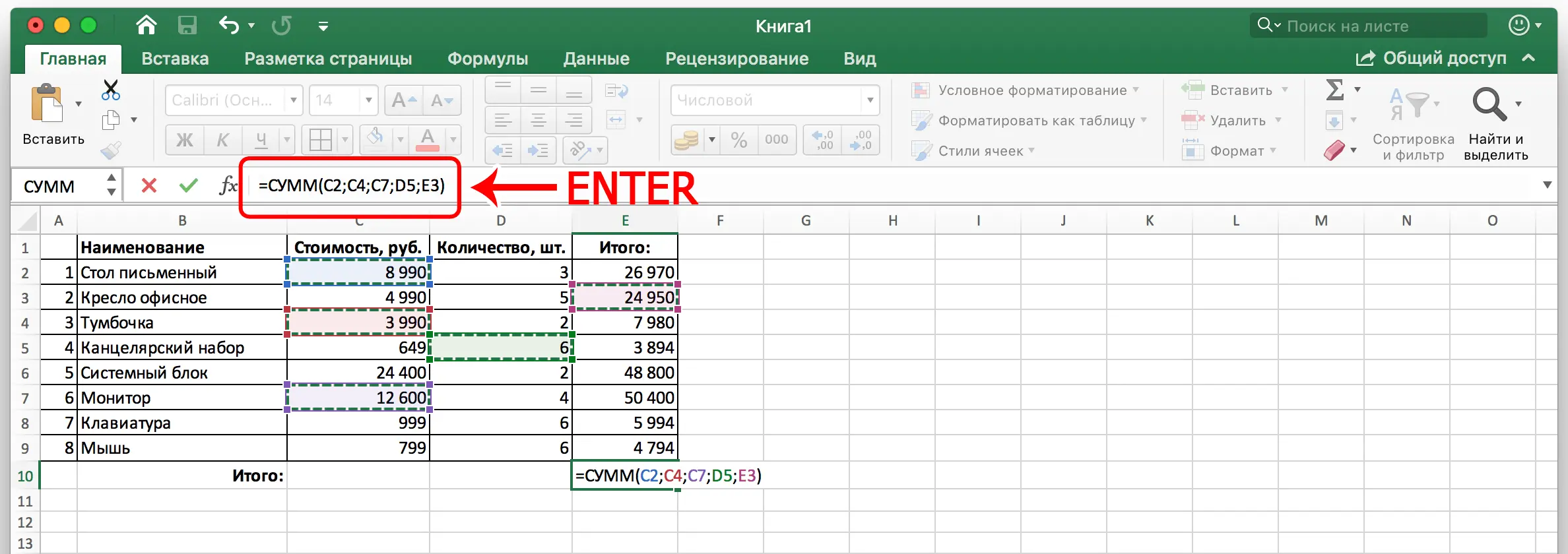
- After all the arguments have been entered, we check that no values have been omitted. After that, close the bracket and press the enter key to confirm the entry of the function.

After that, we get the result of adding the column elements. If an error is found in the final result, then the formula can be adjusted manually. You can use the same delimiters to add some value. If you want to delete a cell that was written by accident, you need to delete it along with the separator that comes before or after it.
Moreover, there is no need to enter the addresses themselves manually. You can select a suitable cell with the left mouse button, and its address will be inserted into the formula automatically. The same goes for ranges. As you can see, there is nothing complicated in summing up the values of the cells that are in the columns. It is enough just to enter the correct formula or use the built-in Excel tool, as a result in your pocket.


