


Contents
This tutorial describes how you can quickly resolve the issue where the Excel VLOOKUP() function shows the user an error in different versions of the spreadsheet program. The most common errors will also be described, as well as recommendations on how to get around the limitations of this function.
Previously, you may have already read about what the function is for. VLOOKUP, and where it can be applied. Especially if you have previously been actively interested in the functions of the Excel spreadsheet program. In this case, you should already become an expert in this field.
But even if you have heard of this feature, you may still run into difficulties. For various reasons, this feature is considered the most complex in a spreadsheet program. There are many limitations to its use, as well as nuances that are imperceptible at first glance, which are the source of a large number of problems and errors.
In this relatively short guide, you’ll find an easy way to work around the #N/A, #NAME, #VALUE! errors that often appear when working with this function, as well as get acquainted with the most common situations when these errors occur.
Several reasons why the #N/A error occurs
In the formula =VPR this error stands for “No data”. In simple terms, the spreadsheet cannot find the value that the user needs. There are many reasons why this problem may appear.
Incorrect entry of the desired value
The most common cause of this error is entering a value with a typo. For example, a letter was accidentally written instead of a number. Especially often this error appears if huge data arrays are processed.
If you are looking for an approximate match
If the user uses range_lookup (that is, interval lookup) as a function argument, a #N/A error may eventually occur. This can happen when one of the following conditions occurs:
- If the value to be found in a particular range is less than the tiniest in the analyzed data set.
- If, before introducing the function, the user did not sort the column associated with it in ascending order.
When searching for an exact match to the entered query
If the value the user is trying to find is searched using a formula and it can’t be found, this can also be the cause of this error.
Column is not leftmost at the moment
The most significant limitation when using the formula VPR – the inability to apply it to a column that is not the leftmost. Usually, the user forgets about this, and as a result, the formula produces the error described above.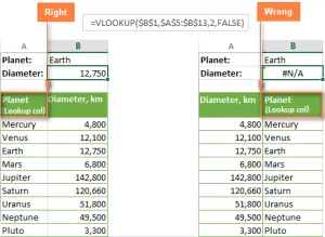
Overcoming this difficulty is as follows: if for some reason it is not possible to move the column to the left, you must use two Excel functions at once: INDEX(), MATCH().
Numeric values are formatted as text
This is also a common source of formula problems. VPR(). Often, the user may not notice that numeric values are formatted as text. Often this problem can occur if information is copied from other sources.
Another reason for this error is that the user forgot that he put an apostrophe in front of the number in order to save the zero that is in front of the value. For example, it may be as shown in the following picture.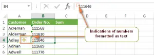
Another reason for the error is that the format may be designated as “General”. You can determine this by the location of the value inside the cell. If they are left aligned, it means that the format is set to General.
To fix this problem, simply click on the “Convert to Number” option in the context menu.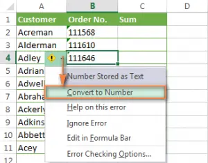
If this error is caused by several cells with numerical values, they must be selected, after which you need to right-click on the corresponding area. In response to this action, a context menu will appear in which you need to select the “Format Cells” option, then you will need to click on “Number” and select a number format. The last step is to click the OK button.
If there is a space at the beginning or end of the content
The cause of this error is the least noticeable. If the table is significantly large, it’s hard to see which cells contain spaces. Especially if some of the cells are outside the screen.
Solution number 1: If spaces are in the table the function is applied to VPR
If gaps are found in the main table, you can use the function TRIM in the Lookup Value argument. It is much easier to demonstrate this with an example.
=VLOOKUP(TRIMSPACES($F2),$A$2:$C$10,3,FALSE)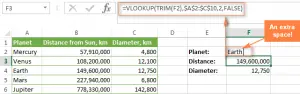
Solution number 2: If the extra spaces are in a column or lookup table
In this case, it will not be easy to prevent the error. Several functions need to be used here: INDEX(), MATCH(), TRIM().
The result is an array formula, for the correct input of which you need to press the key combination Ctrl + Shift + Enter.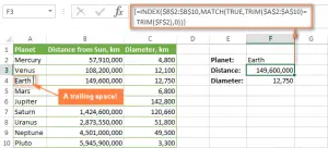
As an alternative way to solve this problem, you can use the Trim Spaces for Excel add-on, which allows you to remove unnecessary spaces in formulas both in the main table and in the lookup table. This is a free tool that can be downloaded from .
Error #VALUE! in the VLOOKUP formula
In general, Excel displays this error if the wrong data type is used in a formula. There are several reasons for this error.
Reason 1: The value you are looking for contains more than 255 characters
This is another limitation of this feature. It cannot be applied to cells whose contents are longer than 255 characters. If this limit is exceeded, the #VALUE! message may appear as a result.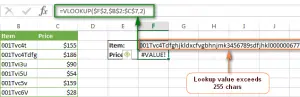
To solve this problem, you need to use a bunch of formulas INDEX()+MATCH(). Here is an example formula that demonstrates the implementation of this task in practice:
=ИНДЕКС(C2:C7;ПОИСКПОЗ(ИСТИНА;ИНДЕКС(B2:B7=F$2;0);0))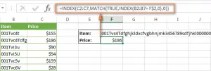
Reason 2: The full path to the workbook used for searching is missing
When specifying data from another file, you must enter the full path to it. Simply put, you must specify both its name and extension, and then enter the name of the sheet and do not forget about the exclamation point. It is best to enclose all this in apostrophes to prevent errors from occurring due to the presence of spaces in the folder to the file or in the Excel workbook itself.
Here’s what that formula looks like:
=VLOOKUP(lookup_value;'[book_name]sheet_name’!table;column_number;FALSE)
Here is an example of using this formula in practice:
=VLOOKUP($A$3;'[New Price.xls]Sheet2′!$B:$C;3;FALSE)
Here the program will look for the contents of cell A3 of column c of Sheet2 of the NewPrice file. The formula will retrieve data from column C.
If the program cannot access the file, the function will return the #VALUE error. Moreover, an error will be generated even if this file is currently open in parallel with the file where the formula is written.
Reason 3: The user entered a value less than 1 in the Column Number argument
It’s hard to imagine that someone could enter a value less than one to designate a column. But this situation happens if the argument contains a variable whose value is calculated by another Excel function.
Thus, if the Column Number argument is less than one, the function will also return the #VALUE!
If the argument “Column number” is greater than the total number of columns in this data set, then the function VPR() will give a #REF! error.
Error #NAME?
The simplest problem is the #NAME? It means that the function name was entered incorrectly. Therefore, in order to correct it, you just need to find a typo.
Why else can the VLOOKUP function not work?
Function VPR() has a rather complicated syntax. But not only it is the cause of difficulties in working with this formula. In the course of using the program, many troubles can appear even in seemingly simple cases. The following are the most common situations where VLOOKUP() can throw an error. It also describes the limitations that need to be taken into account.
Case insensitive
This function cannot figure out which is the capital letter and which is the small letter. Therefore, in a data set where there are elements that are similar except for the case of characters, it will return the first one that comes across, case insensitive.
To solve this problem, you can use another Excel function that can look up the desired value in a column (INDEX(), MATCH(), LOOKUP(), and others) along with EXACT(). The last function can distinguish case.
Returning the first value found
In addition to using a different function to find a case-sensitive value, you can use a different formula if you know exactly which value to look for in order. To do this, you need to use the functions INDEX(), SMALL() и LINE(). So it will be possible to choose 2, 3, 4 or any other required value.
A new column has been inserted into or removed from the table
Unfortunately the formula VPR() stops working every time a column is added to the table. This is because its syntax requires the introduction of the entire array of cells in which information is searched. Of course, the situation changes if a column is inserted there.
Here you also need to use the INDEX() and MATCH() functions. They allow you to specify not an array of the entire range, but only the required columns, and therefore you can edit all the others without having to update the formulas associated with them.
Cell reference corruption when copying a function
It immediately became clear to you what the problem was, right? Solving it is simple: using absolute references to those cells that need to be left stable when copying the function. To do this, put a dollar sign ($) in front of the column or row name. For example, write a range like this: $A$2:$C$100. An easier option: $A:$C. Using the F4 key, you can quickly change the cell address type.
Handling errors when using the VLOOKUP function
If you don’t need to display an error code to users (for example, #N/A), you can use VPR() together with the function IFERROR() in Excel latest versions up to 2007. You can also use the two IF()+ISERROR() functions if the version is older.
Using the IFERROR function
This formula has a simple syntax:
IFERROR(value; value_if_error)
Thus, in place of the first argument, a value is inserted that is tested for an error, and in place of the second argument, it is necessary to write the text or number returned when an error occurs.
Here is an example of using the function in practice:
=IFERROR(VLOOKUP($F$2,$B$2:$C$10,FALSE),””)
In this case, an empty cell will be returned if an error is found.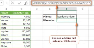
You can write any other phrase in quotation marks. For example, the one shown in the screenshot.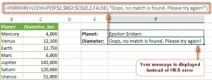
Using the ISERROR function
The function described above first appeared in the Excel 2007 version, therefore, if older versions of the program are used (for example, if the computer has a small performance, but it needs to process large amounts of data), you need to use this formula:
=IF(ISERROR(VLOOKUP formula),”Your error message”,VLOOKUP formula)
In practice, the formula will look like this:
=ЕСЛИ(ЕОШИБКА(ВПР($F$2;$B$2:$C$10;2;ЛОЖЬ));»»;ВПР($F$2;$B$2:$C$10;2;ЛОЖЬ))
So, that’s all for today. As you can see, most of the problems with the formula VPR are complex at first glance. In fact, they are solved quite simply. It is enough to remember what each of the errors means, and next time you can understand what actions to take. If the spreadsheet is going to be read by a user who doesn’t understand spreadsheets at all and still can’t fix the error, you can program the text that will be displayed instead of the error code.