


Contents
Many users are faced with the problem of why, when trying to sum a number, they fail to do so. Well, let’s look at the causes of this problem in more detail. Most often this is due to the fact that the number was stored in text format. Today we will find the causes of this phenomenon, and also learn how to solve it with different methods.
Possible reasons why the amount is not considered
Very often, the amount does not want to be considered after data from other programs has been copied to Excel. And in the course of using this information, it turns out that the numbers cannot be summed up, and between dates it is not possible to understand how many days have passed.
Number saved as text
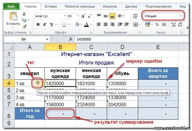
How can you tell if a number has been stored in text format? To do this, you need to look at which edge the number was pressed against. In addition, when importing data, a green triangle may be displayed, which indicates an error in converting data into the correct format. If you hover over it with the mouse, it will show that the number was written in text format.
Ways to solve the problem
At the same time, if you try to change the cell format using standard Excel tools, then nothing will work. True, if you put the text input cursor in the formula input field, then press the “Enter” button, then the problem is solved. But obviously. that this is a very inconvenient method when it comes to a huge number of cells.
True, there are many other ways to get out of this situation.
Error marker and tag
First of all, you can directly use the marker that signals an error. If there is a green tag on the cell, then by clicking on it, it becomes possible to immediately turn it into a text format. To do this, in the menu that appears, click on “Convert to Number”.
Operation Find/Replace
Another method for dealing with a situation in which numbers are written in text format is to use the Find / Replace operation. Let’s say some cells contain a number that has a decimal point, stored in text format. To do this, click the appropriate button on the ribbon or in the top menu (depending on the version of Excel you are using). A window will appear in which you need to replace the comma with itself. Yes, literally, you need to enter a comma in the “Find” field and also enter a comma in the “Replace” field. After that, the format should be converted automatically. In principle, the operation is similar to clicking on the formula bar and then pressing the enter button. The same operation can be with dates, only you need to replace the dot with a dot.
If the data was imported from other programs, then the reason may also be the difference in the formats of decimal values. If a cell uses a dot instead of a comma as a separator, then Excel will not recognize this data as numeric. In this case, you need to replace the dot with a comma in the corresponding cells.
Paste special
Using “Paste Special” is a fairly universal method, since it allows you to turn any numbers related to any kind, both fractional and integer, into a number format. It can also be used to convert dates to the appropriate format. To use this function, you need to find any empty cell, select it and copy it. After that, right-click on any cell whose format is incorrect, after which we press the buttons “Paste Special” – “Add” – “OK”. This is the same operation as adding zero. The value of the cell does not change absolutely, but its format is converted to numeric. You can also use multiplying a range of values by one.
Text by Columns tool
This tool is most useful when using only one column. If there are more, it’s okay, but you will have to use it separately for each column. To do this, you need to select the corresponding column, set the number format and execute the “Text by Columns” command, which is located in the “Data” tab.
formula
A very popular way to solve problems with displaying cells is to use the function SUBSTITUTE(), SIGNIFICANT() and some other formulas. This method can be used if it is possible to use additional columns in which the formula can be entered. You can use other mathematical operations, such as double minus (-), adding zero to a number, multiplying by one, and any other similar operation. After that, the resulting cells are copied and pasted into the places where previously there were values in text format.
Macros
Special attention should be paid to the use of macros to correct errors. In principle, you can use any previous method through a macro, so we will give it separately. It is enough just to write the corresponding script and execute it. Here are some examples that you can use.
Sub conv()
Dim c As Range
For Each c In Selection
If IsNumeric(c.Value) Then
c.Value = c.Value * 1
c.NumberFormat = «#,##0.00»
End If
Next
End Sub
This code multiplies the text value by one.
Sub conv1()
Selection.TextToColumns
Selection.NumberFormat = «#,##0.00»
End Sub
And this is the code that demonstrates the use of the Text in Columns tool.
There are extraneous characters in the number entry
Ways to solve the problem
Also, a common reason why numbers start to appear as text is the appearance of invisible characters in the corresponding cells. Most often they are spaces, which can be anywhere from the beginning and end of a number to being used to separate digits from each other.
Another type of space that can prevent a cell from being saved in the correct format is the so-called non-breaking space (which has the code 160). The method described above is not enough to solve this problem. To solve the problem, you need to copy this character directly from the cell, and then paste it into the “Find” field, or type Alt + 0160 in this field (but this number will not work on laptops, because a numeric keypad is required to complete this task) .
For an ordinary person, it is generally not always clear what a non-breaking space is and where it can be used. To make it clearer, let’s look at this text.

At first glance, nothing special. But if a person has worked at least a little with texts, he will immediately understand that the breakdown of this fragment into lines is far from successful. Let’s take a closer look at it. For example, the initials and surname were separated, which is not very good. The same goes for the year number and the year abbreviation.
The separation of the surname “Palazhchenko” and the designation of his position also turned out to be unsuccessful. As a result, this piece of text began to look like direct speech.
In simple words, this fragment contains pieces where a space should be used. But as a result of this gap, the accuracy of the design is lost. And to achieve this, you need to use the non-breaking space character. With it, we also separate words, but they remain on the same line. The words separated by it are perceived by the program as one whole word, but at the same time they look like several. It turns out a kind of compromise between how the text is displayed and how it is perceived by the program. That is, if it turns out that they need to be transferred to a new line, then they will all be transferred. They should be used in the following situations:
- Before a dash that is in the middle of a line. Only in three cases is it allowed to use a dash at the beginning of a line: if direct speech is used, if the dash marks an element of the list, and provided that the dash replaces the dash. To prevent a dash from wrapping to a new line, it must be preceded by a non-breaking space.
- Between a number and a unit of measure. Quite often this problem happens. As a result, a person can transfer a number with a non-breaking space to an Excel table, and the unit of measure will be in another cell. In general, you should use a non-breaking space in this case so as not to separate them. But when transferring to Excel, problems may arise.
- before the percent sign. In this case, the cell may not be converted to percentage format. Of course, not everywhere you can find the percent sign, separated from the number by a space, but some believe that this is correct. Therefore, when transferred to Excel, data can be displayed in text format. The same goes for regular space.
- Number and paragraph sign. This situation also often arises when you have to move sections of textbooks or parts of documents into spreadsheets.
- Multi-digit numbers. The most common reason why non-breaking spaces wrap into an Excel spreadsheet. According to the rules, spaces are required in multi-digit numbers to make them easier for users to read. But if the number is too large, then it can automatically be transferred in parts to the next line. To solve this problem, a non-breaking space is used. And if such a number is copied into a cell, it will automatically be displayed in text format.
Typically, non-breaking spaces end up in Excel after the data has been transferred from a Word document.
There is no way to easily detect non-breaking spaces using Excel. But if you copy the contents of the cell in Word and enable the option to display non-printable characters, you can see peculiar circles that look like a degree sign, only a little larger. It’s just these gaps.
This symbol is in any font. As a rule, all programs designed to work with text process it correctly. However, some of them have non-breaking spaces of the same size. Because of this, there are problems with displaying the page in width, since regular and non-breaking spaces have the same dimensions.
You may need to enter a non-breaking space in Excel as well. To do this, you need to press the key combination ALT and 0160. Windows also comes standard with the hot key combination CTRL + SHIFT + SPACEBAR, with which you can enter a non-breaking space in almost any program.
There are two main ways to solve this problem – use the Find / Replace function or use a formula.
Operation Find/Replace
To remove spaces, you can use the Find / Replace function. Enter a space character in the first field, while leaving the bottom field blank.
It is important to make sure there are no spaces.
Formula
Using a formula is also possible to remove spaces. Depending on whether the space is regular or non-breaking, you need to use different formulas. There is also one universal one that allows you to remove all the spaces contained in the cell at the same time.
What are these formulas?
In all cases, the function is used SUBSTITUTE. If we need to remove the usual space, then the following formula is used.
=—SUBSTITUTE(B4;” “;””)
With the help of a double minus sign, we convert a text value into a numeric value. This is equivalent to multiplying the resulting number by -1, and then multiplying the resulting negative value by -1 again. As a result, nothing has changed, but thanks to the performed mathematical operation, the cell is automatically converted to a number format.
In the case of non-breaking spaces, the formula will be as follows.
=—SUBSTITUTE(B4,CHAR(160),””)
As you can see, here we use the character code as the second argument. And with the help of this formula, you can remove both ordinary and non-breaking spaces.
=—SUBSTITUTE(SUBSTITUTE(B4,CHAR(160),””);” “;””)
Sometimes the problem is much more complicated than it might seem at first glance. Therefore, in some cases it is necessary to combine all the methods described above.
Conclusions
Thus, the problem of why it is impossible to sum several numbers is not as difficult as it might seem at first glance. Solving it is very simple, just knowing some Excel functions is enough.