Where is the Chart Wizard in newer versions of Excel

Microsoft Corporation removed the chart wizard from the latest editions of their program, since Excel 2007. The company decided to completely change the approach to working with charts and implemented a new settings system, so the master has lost its relevance.

Those who are used to adding graphics to a document using the old functionality may not like this solution, however, the new option is much easier to use and more convenient to use. 

The innovation is tightly integrated into the ribbon interface of the application and allows you to see the changes made at each stage of the configuration using the preview function. This approach makes it possible to choose the most suitable parameters immediately before inserting the chart into the document.  

Comparison of the diagram wizard with the new customization system 

If you are accustomed to using the wizard, then you should not be disappointed. The updated functionality of the program in most cases allows you to easily configure the chart settings in just a couple of mouse clicks. 

Let’s compare the capabilities of the new insert method with the Chart Wizard in detail.

To insert a chart in older versions of Excel, the wizard offered to set four parameters of the created element:

1. Chart type. Before specifying the data for plotting, it was necessary to select the appearance of the graph. 
2. In the next stage selected cells with numbersand the type of data visualization was configured using columns or rows.
3. Thereafter label settings changed on the axis scale.
4. Finally, the user indicated where should the chart be placed – insert it on the current sheet or create a new one. 

If you needed to change the settings of an existing chart, you could find them in the wizard or pop-up menus, as well as on the formatting tab. 

Starting with Excel 2007, the Chart Wizard has been replaced with a more convenient chart customization option that provides the user with more options. Consider how the process of creating a diagram is going on now.

1. At the first stage, the user immediately selects cells with data for plotting. In this way, you can see how the diagram will look with the available parameters before the end of the full setup.
2. Chart type. Using the “Insert” tab, you can select the type of graph you want by clicking on the appropriate option. Various variations of the chart will appear on the screen. By hovering over the sample, you can immediately see what the graph will look like. After the user selects the desired subview of the graph, it will immediately appear on the sheet.  
3. Rapid change in design and format. If you need to modify an existing chart, you just need to mark it and use the three new tabs on the toolbar − “Constructor”, “Layout” и “Format” (there may be less depending on the version of the program). This feature allows you to select several professional presets in one click to customize an existing chart.  
4. You can now change chart parameters, such as labels and axes options, simply by calling the element’s context menu and selecting the appropriate option. 

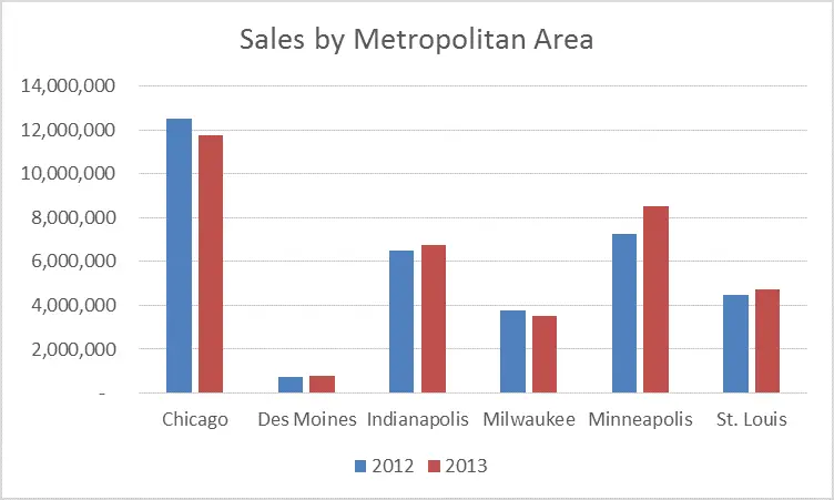
Let’s consider further the options for setting up a bar chart in different versions of Excel in detail: 

Download the attached document with an example table. Our file shows relative sales data by city:

To create such a table in Excel version 1997-2003, you will need to do the following:

1. Click on the Add Chart button. 
2. Select the histogram and in the view selection window click on the first option. 
3. Push the button “Further”.
4. In the next window for the range, select cells B4: C9 (marked in light blue in the file).
5. For rows, select the option “columns”.
6. Go to the tab “View” and for labels along the X axis, select cells A4: A9.
7. Push the button “Further”.
8. In a new window, set the name of the chart and add a legend.
9. After that, by clicking “Further”, indicate the placement of the graph on the existing sheet. 

To create a similar chart in the 2007-2013 versions of Excel, you will need to do the following:

1. Select cells with mouse B4: C9 (light blue).
2. Go to the tab “Insert” and click on the add histogram button.
3. Select the first option from the menu.
4. Now in the data section, click on the button “Select data”.
5. In the appeared window for signatures on the horizontal axis, set the range A4: A9 using the button “Change”.
6. For the name of the first row, select a cell B3, and for the second C3.
7. We click on the button «OK».
8. Double click on the title of the chart and change the title.

Additional settings

Take some time to familiarize yourself with the advanced chart settings. Open a tab “Format” and experiment with the options. Most of the options have a preview function, and their names will tell you exactly what will change as a result of applying the option.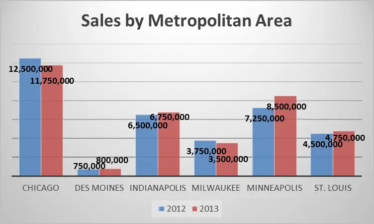

As you know, the best way to learn something is to try it yourself!