


In this lesson, we will learn about the function VIEW, which allows you to extract the information you need from Excel spreadsheets. In fact, Excel has several functions for finding information in a workbook, and each of them has its own advantages and disadvantages. Below you will find out in which cases it is necessary to use the function. VIEW, consider a few examples, and also get acquainted with its recording options.
Options for recording the VIEW function
Let’s start with the function VIEW has two notation forms: vector and array. When you enter a function on a worksheet, Excel reminds you of this in the following way:
Array form
The shape of an array is very similar to functions VPR и GPR. The main difference is that GPR looks for the value in the first row of the range, VPR in the first column, and the function VIEW either in the first column or in the first row, depending on the dimension of the array. There are other differences, but they are less significant.
We will not analyze this recording form in detail, since it has long been outdated and left in Excel only for compatibility with earlier versions of the program. Instead, it is recommended to use the functions VPR or GPR.
vector shape
The LOOKUP function (in vector form) scans a range that consists of one row or one column. Finds the given value in it and returns the result from the corresponding cell in the second range, which also consists of one row or column.
Blimey! Well, it’s necessary to write this … To make it clearer, consider a small example.
Example 1
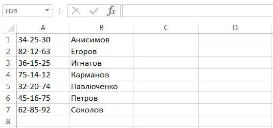
The figure below shows a table with phone numbers and names of employees. Our task is to determine the phone number by the name of the employee.
In this example, the function VPR do not apply because the column being viewed is not the leftmost column. In such cases, you can use the function VIEW. The formula will look like this:
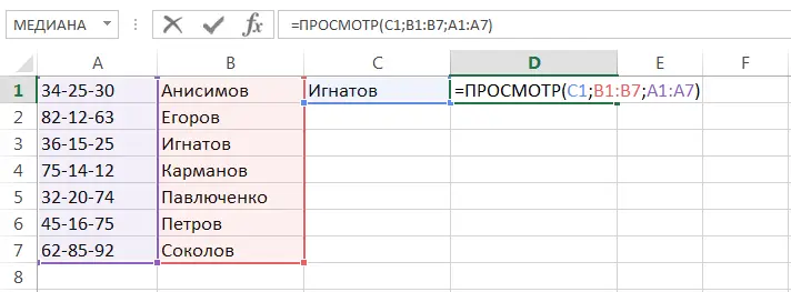
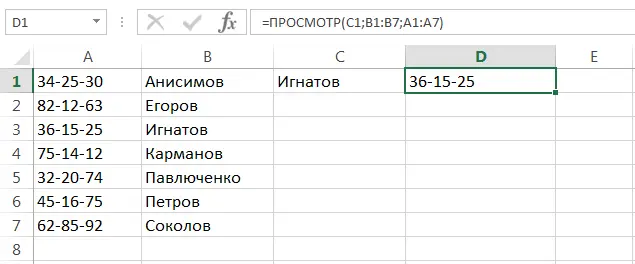
Function first argument VIEW is cell C1, where we indicate the desired value, i.e. surname. The range B1:B7 is a lookup range, also called a lookup vector. From the corresponding cell in the range A1:A7, the function VIEW returns a result, such a range is also called a result vector. Clicking Enter, make sure everything is correct.
Example 2
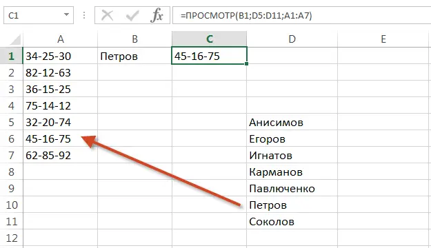
Function VIEW in Excel, it is convenient to use when the view and result vectors belong to different tables, are located in distant parts of the sheet, or even on different sheets. The most important thing is that both vectors have the same dimension.
In the figure below you can see one such example:
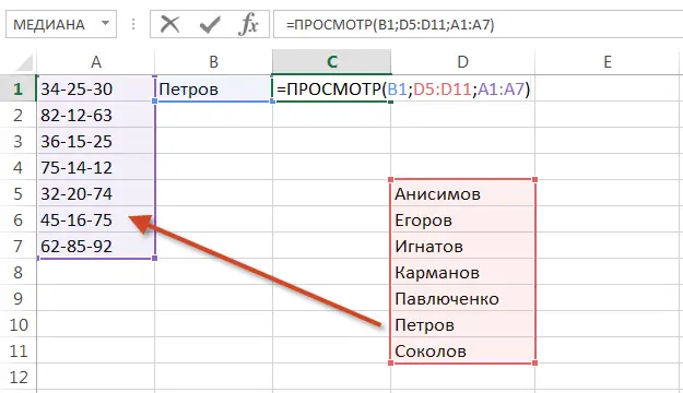
As you can see, the ranges are offset from each other, both vertically and horizontally, but the formula will still return the correct result. The main thing is that the dimensions of the vectors match. Clicking Enter, we get the desired result:
When using the function VIEW in Excel, the values in the lookup vector must be sorted in ascending order, otherwise it may return an incorrect result.
So, briefly and with examples, we got acquainted with the function VIEW and learned how to use it in Excel workbooks. I hope that this information was useful for you, and you will definitely find a use for it. All the best to you and success in learning Excel.