


Contents
There are many areas where a trend line can be used. But the most popular of them, of course, are the financial markets. In business, too, it is used quite often to compile reports and predict possible prospects for the development of a project or a company as a whole.
It will also be a useful tool in those areas of human activity where you can make forecasts based on statistical data. And there are many more such areas than it might seem at first glance. In particular, these include sociology, psychology, programming (the use of mathematical models makes it possible to automate the forecasting process), and so on. This is especially useful in combination with a qualitative analysis of information.
The main problem with almost any graph with a lot of information is that the readings in it are very variable. Therefore, there may be a large amount of data that makes it difficult to understand what is really the trend observed in this industry.
The trend line is a classic statistical tool that allows you to predict, without much experience, in which direction the target indicator will move after some time and at what point it will be. It also makes it possible to indirectly determine the factors that influence the formation of this trend. True, this cannot be done by purely statistical methods, you need to understand the fundamental patterns that affect the formation of a trend.
How to add a trend line to an Excel chart
The trend line makes it possible to understand the current trends of a certain indicator. And since this tool is now especially often used in financial markets, we will use this example.
The trend line in the financial markets is a classic tool for analyzing the dynamics of quotations, which has been used since the creation of the first stock exchange. But it alone is not enough, and now more and more new technical indicators are being developed that can significantly improve the quality of forecasts. There is also a separate category of indicators that allows you to directly anticipate a trend reversal. At the same time, the trend line makes it possible only to state the current price direction.
Therefore, it is recommended to use a trend line in conjunction with oscillators. This is a category of technical indicators that has time to notice a trend change before the trend line does.
Creating a trend line is possible using standard Excel tools. It is still actively used, so you need to be able to build it. Let’s see how to do it.
Graphing Process
For the process of plotting a trend line to be successful, the chart must fit the mathematical function. To create a graph, you need to follow this algorithm:
- Select the set of cells of interest.
- Go to the toolbar (or, as they often say, the ribbon) to the “Home” tab, and find the “Charts” button there.
- Then you need to select “Dotted”, and then “Dotted with smooth lines and markers”.
After the user clicks on the chart, he will be able to use another panel through which the trend line is added to the chart.
Creating a trend line
So, let’s move on to the Chart Tools panel. There is the “Layout” tab, through which the trend line is added to the chart. After we press the button of the same name, it will be possible to choose the approach method. You need to choose a linear type. Then a black line will appear, which will express the current trend.
It is important to understand that some types of charts do not support a trend line. Therefore, it is recommended to use the most standard ones.
All other types of charts make it possible to add a trend line to them.
Setting lines
The next step is setup. First you need to add an equation to the graph. This is done by double-clicking the left mouse button on the diagram. The user then needs to select the “Show Equation on Chart” option.
If there is more than one graph on the diagram, then you need to choose the most suitable one for forecasting.
You need to remember the following points if you need to adjust certain parameters of the trend line:
- To name a chart, double-click on it. The title is written in a small input field. To locate the chart title, open the Chart Tools tab again, then select Layout and Chart Title. A list of possible header locations will pop up.
- This section contains a setting that allows you to set the titles of the axes and their place on the chart. The important thing is that the user has the right to position the title directly along the X or Y axis. This makes it possible to make the appearance as readable as possible.
- To make changes immediately in the lines, you need to open the “Layout” tab and go to the “Analysis – Trend Line” items there. And if you click on “Advanced Options”, a window will open in which you can customize the trend line – adjust its format, edit color, smoothing, and a number of other parameters.
- You can also check the trend line for veracity. To do this, you need to enable the option “Place approximation confidence value on the chart” and close the window. The most optimal value is 1. If deviations are observed, this indicates the degree of reliability of the constructed statistical model.
Prediction
The most accurate forecasts are possible if you make the graph type “histogram”. This makes it possible to match the equations. To do this, you need to follow this algorithm:
- Open context menu. In this list, click on the item “Change chart type”.
- The settings window will open. There, the type “Histogram” is selected, and then we select the variety.
The user can now see both graphs. They contain the same information but provide more accurate forecasts because each type of chart uses a different equation to plot the trend line.
Next, we are faced with the task of comparing different charts. To do this, you need to enable visual display. To do this, the following steps are performed:
- The histogram format changes to the simple scatter plot we did earlier. To do this, you need to use the “Change Chart Type” item.
- Double click on the trend line to change the forecast parameters to 12 and save the changes made.
With these parameters, you can see that the angle of the trend line differs depending on the chart used, but still the direction does not change. From this we can conclude that it is not enough to use only one trend line to make reliable forecasts in the financial markets.
When it comes to trading in financial markets, the use of technical indicators (which the trend line is) is not enough. It is also necessary to understand the fundamental laws of the economy and the general qualitative trends in the development of the industry. Otherwise, even with a high confidence factor, the real accuracy of the forecasts will suffer greatly.
Trendline Equation in Excel
Just adding a trend line is not enough, you also need to be able to choose the right equation so that the data is displayed as correctly as possible. It is possible to determine which of them is correct, focusing on the reliability number. If the value differs from one, then the chart has been configured incorrectly. Accordingly, you need to display the graph differently or use other equations for the calculation.
Linear approximation
Let’s take the following case: an employee entered into transactions for ten months, and every month he made a certain number of them.
The chart will be built based on this data. You just need to follow some steps, namely:
- Adding a trend line to a chart.
- Adding an equation to the chart that is used to analyze the trend and confidence value. Both of these values play a huge role in predicting the dynamics of any indicators.
Suppose we have a chart where data is entered and the type of chart display is selected, in which the reliability is 0,9929, and based on the chart data, we can conclude that the employee works more than before. In this case, using the chart, you can determine how many trades are expected to be made in the future. To do this, you need to insert the period number into the used formula.
Exponential trend line
This type of trend line is now familiar to many. All pandemics develop according to this scenario, as well as a number of other processes. A characteristic feature of this type of trend line is that the numbers are constantly increasing exponentially. For example, 1,2,4,8 and so on. According to a similar scenario, epidemics develop precisely, since the more sick, the more people the disease can be transmitted.
We will try to abstract ourselves from unpleasant things and move on to other areas, for example, business.
Let’s say you are managers who need to analyze how much energy was released over a certain period. Conditional values will be used, which may differ from reality. Just to show an example.
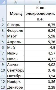
Now, based on these data, we perform the construction of a graph. Next, add an exponential trend line.
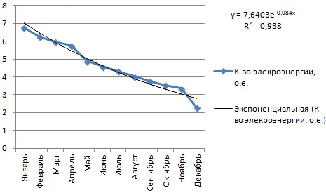
The trend line confidence in our example is 0,938, which means that the probability of error is quite low. Therefore, the forecasts can be trusted.
logarithmic trend line
It is used in situations where indicators can change dramatically. For example, at first there is a rapid growth, after which there is a period of stability. Using a logarithmic trend line, you can try to predict how successful sales of a product that has just appeared will be.
First, the company needs to attract new customers. Therefore, growth will be rapid. Further, the reliance goes primarily to making those who have already been attracted loyal to oneself. Consequently, the point of application of efforts changes and, accordingly, the growth of the client base is adjusted.
Let’s make such a graph for this example.
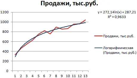
In this case, the approximation error is also minimal, so the information obtained can be trusted. Now let’s try to guess how intense sales will be in the future. To do this, you need to substitute the number of the corresponding period as the value of the variable x.
Alternatively, the following table with predictions is possible.
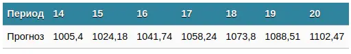
In our case, in order to roughly understand how products will be sold in the future, the following formula was applied: =272,14*LN(B 18)+287,21. Where B18 is the period number.
Polynomial Trendline in Excel
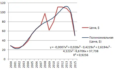
This trend line is typical for volatile (changeable) indicators. It is very good to use it for trading cryptocurrencies or other high-risk assets.
A trend line of this type is characterized by either an increase or a decrease in indicators in a fairly wide range. Its use is also possible for processing huge amounts of information of a quantitative type. Especially this trend line is often used when there are a large number of extremes on the chart (that is, lows and highs).
The oil price chart is the most convenient way to demonstrate how this model works. In order for the reliability value to be close to one, the sixth degree had to be set. But such a trend line makes it possible to make fairly accurate forecasts.
Conclusions
Drawing a trend line is a fairly simple procedure. But data analysis with its use is already a more difficult task. But with the help of built-in Excel tools, you can make effective forecasts for the development of a wide variety of indicators from different areas. And although the use of a trend line is mostly automated in modern programs, it may sometimes be necessary to use Excel for this purpose.
In general, one trend line is not enough to make effective forecasts. This is not a panacea, and one should not hope that such an elementary mathematical model can work wonders. However, it is one of the simplest elements of statistical analysis. And now you know how to use it in real work.